Programming Session 3

Goals

1. Plotting graphs using matplotlib

2. Reading and plotting image histograms.

3. Working with clustering and classification algorithms

Exercise 1 [★]

matplotlib can be used to plot graphs. Given below is a very simple code with only x values. After importing the matplotlib library, we initialize x values and plot it.

import matplotlib.pyplot as plot

x = [1, 2, 3, 4, 5, 6, 7, 8, 9, 10]
plot.plot(x)
plot.show()

Now let’s change the color, style and width of the line.

import matplotlib.pyplot as plot

x = [1, 2, 3, 4, 5, 6, 7, 8, 9, 10]
plot.plot(x, linewidth=3, drawstyle="steps", color="#00363a")
plot.show()

We will now initialize the y-values and plot the graph.

import matplotlib.pyplot as plot

x = [1, 2, 3, 4, 5, 6, 7, 8, 9, 10]
y = [0, 1, 0, 0, 1, 0, 1, 1, 1, 0]
plot.plot(x, y, linewidth=3, drawstyle="steps", color="#00363a")
plot.show()

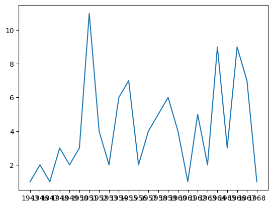
In the first practical session, we saw how to parse JSON files. Continuing with the same JSON file, we will now plot the results of number of programming languages released per year. Verify the output.

from pandas import json_normalize
import pandas as pd
import json
import matplotlib.pyplot as plot

data = json.load(open("../data/pl.json"))
dataframe = json_normalize(data)
grouped = dataframe.groupby("year").count()
plot.plot(grouped)
plot.show()

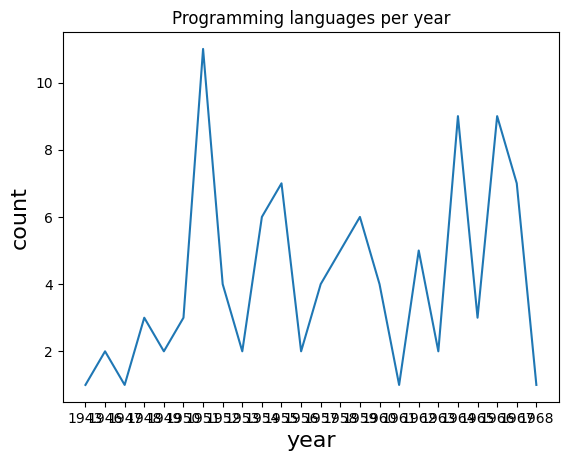
Following program will add title and labels to the x-axis and y-axis.

from pandas import json_normalize
import pandas as pd
import json
import matplotlib.pyplot as plot

data = json.load(open("../data/pl.json"))
dataframe = json_normalize(data)
grouped = dataframe.groupby("year").count()
plot.plot(grouped)
plot.title("Programming languages per year")
plot.xlabel("year", fontsize=16)
plot.ylabel("count", fontsize=16)
plot.show()

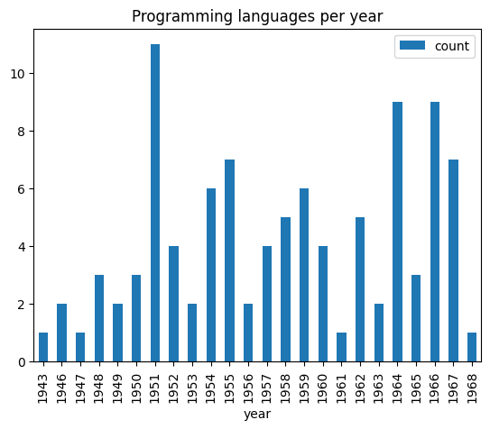
There is yet another way to plot the dataframes, by using pandas.DataFrame.plot.

from pandas import json_normalize
import pandas as pd
import json
import matplotlib.pyplot as plot

data = json.load(open("../data/pl.json"))
dataframe = json_normalize(data)
grouped = dataframe.groupby("year").count()
grouped = grouped.rename(columns={"languageLabel": "count"}).reset_index()
grouped.plot(x=0, kind="bar", title="Programming languages per year")

<Axes: title={'center': 'Programming languages per year'}, xlabel='year'>

Now, we want to create multiple subplots. A simple way is given below. Recall in first practical session, we did group by on multiple columns. Subplots can be used to visualize these data.

from pandas import json_normalize
import pandas as pd
import json
import math
import matplotlib.pyplot as plot

jsondata = json.load(open("../data/plparadigm.json"))
array = []
for data in jsondata:
    array.append([data["year"], data["languageLabel"], data["paradigmLabel"]])
dataframe = pd.DataFrame(array, columns=["year", "languageLabel", "paradigmLabel"])
dataframe = dataframe.astype(
    dtype={"year": "int64", "languageLabel": "<U200", "paradigmLabel": "<U200"}
)
grouped = dataframe.groupby(["paradigmLabel", "year"]).count()
grouped = grouped.rename(columns={"languageLabel": "count"})
grouped = grouped.groupby(["paradigmLabel"])
# Initialization of subplots
nr = math.ceil(grouped.ngroups / 2)
fig, axes = plot.subplots(nrows=nr, ncols=2, figsize=(20, 25))
# Creation of subplots
for i, group in enumerate(grouped.groups.keys()):
    g = grouped.get_group((group,)).reset_index()
    g.plot(
        x="year", y="count", kind="bar", title=group, ax=axes[math.floor(i / 2), i % 2]
    )
plot.show()

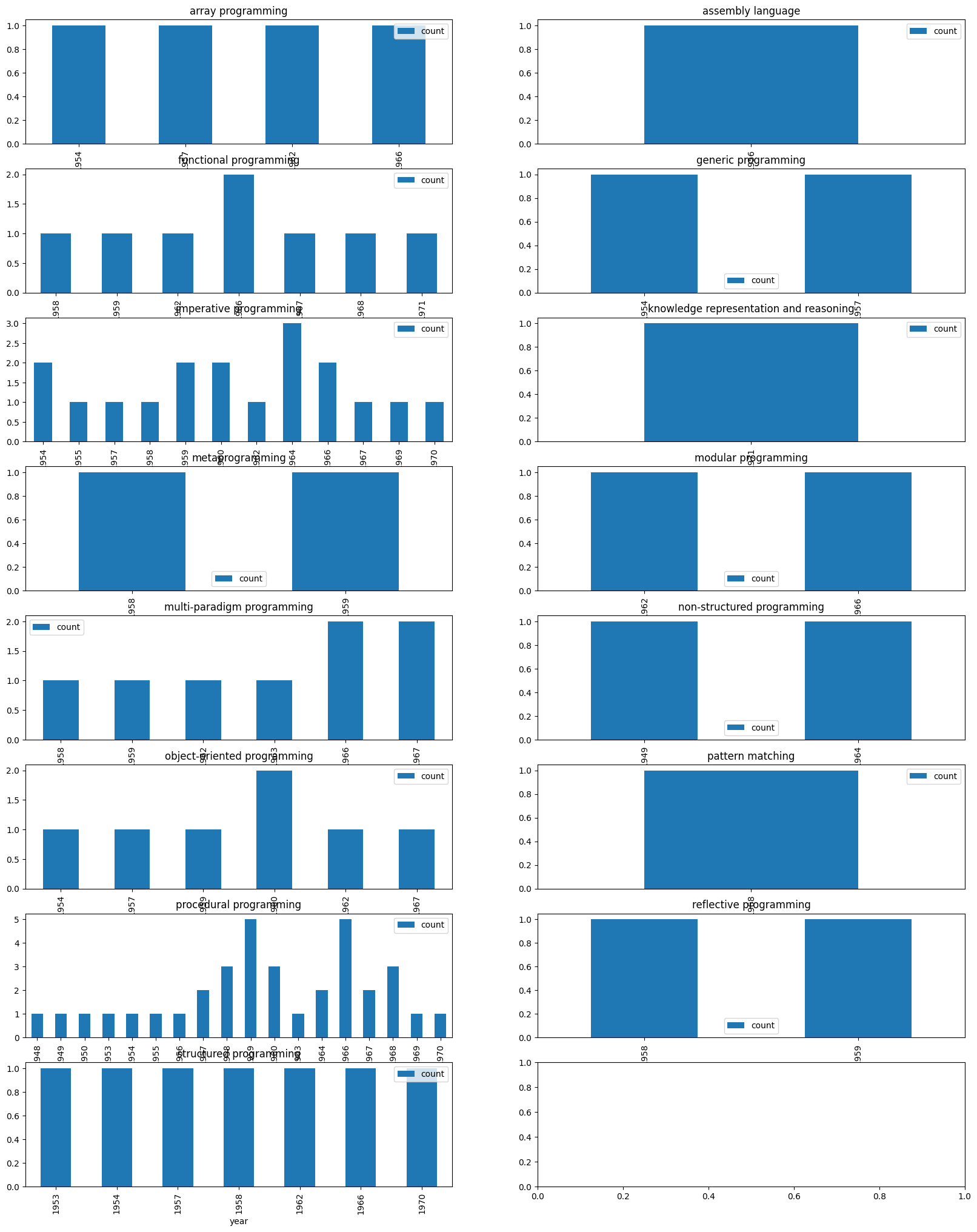
Make changes to the above code, so that we can get visual information on count of languages of different programming paradigms released in every available year, i.e, for each year, we want to see the count of programming languages belonging to each programming language paradigm.

Exercise 2 [★]

In this exercise, we will work on images. Download an image (e.g., picture.bmp and flower.jpg) in your current working folder and open it in the following manner. We will first try to get some metadata of the image.

import os, sys
from PIL import Image

imgfile = Image.open("../images/picture.bmp")
print(imgfile.size, imgfile.format)

(640, 480) BMP

We use Image module of Python PIL library (Documentation). We will now try to get data of 100 pixels from an image.

import os, sys
from PIL import Image

imgfile = Image.open("../images/flower.jpg")
data = imgfile.getdata()
for i in range(10):
    for j in range(10):
        print(i, j, data.getpixel((i, j)))

0 0 (102, 94, 105)
0 1 (77, 69, 82)
0 2 (77, 70, 86)
0 3 (75, 71, 86)
0 4 (75, 71, 86)
0 5 (77, 71, 85)
0 6 (78, 70, 83)
0 7 (80, 70, 81)
0 8 (78, 70, 83)
0 9 (80, 69, 83)
1 0 (78, 70, 83)
1 1 (53, 45, 58)
1 2 (53, 46, 62)
1 3 (50, 46, 61)
1 4 (53, 46, 62)
1 5 (52, 46, 60)
1 6 (53, 45, 58)
1 7 (55, 45, 56)
1 8 (55, 44, 58)
1 9 (54, 43, 57)
2 0 (76, 70, 82)
2 1 (53, 45, 60)
2 2 (53, 45, 60)
2 3 (52, 46, 60)
2 4 (53, 47, 61)
2 5 (54, 46, 59)
2 6 (55, 44, 58)
2 7 (56, 44, 58)
2 8 (54, 44, 55)
2 9 (54, 42, 54)
3 0 (78, 72, 86)
3 1 (55, 47, 62)
3 2 (56, 48, 63)
3 3 (55, 47, 60)
3 4 (56, 48, 61)
3 5 (57, 46, 60)
3 6 (56, 45, 59)
3 7 (56, 44, 58)
3 8 (54, 42, 54)
3 9 (53, 41, 53)
4 0 (80, 74, 86)
4 1 (57, 49, 62)
4 2 (57, 49, 60)
4 3 (57, 49, 60)
4 4 (59, 49, 60)
4 5 (57, 47, 56)
4 6 (56, 44, 54)
4 7 (56, 43, 53)
4 8 (54, 41, 51)
4 9 (52, 39, 49)
5 0 (82, 76, 90)
5 1 (59, 51, 64)
5 2 (61, 50, 64)
5 3 (59, 49, 60)
5 4 (58, 48, 57)
5 5 (57, 45, 55)
5 6 (55, 43, 53)
5 7 (54, 41, 51)
5 8 (53, 40, 50)
5 9 (52, 39, 49)
6 0 (84, 76, 91)
6 1 (61, 50, 66)
6 2 (61, 50, 64)
6 3 (59, 47, 59)
6 4 (58, 46, 58)
6 5 (56, 44, 56)
6 6 (54, 42, 54)
6 7 (52, 40, 52)
6 8 (51, 40, 46)
6 9 (51, 40, 46)
7 0 (83, 75, 90)
7 1 (61, 50, 66)
7 2 (61, 48, 65)
7 3 (58, 46, 60)
7 4 (56, 44, 56)
7 5 (54, 42, 52)
7 6 (53, 41, 51)
7 7 (51, 39, 49)
7 8 (52, 41, 47)
7 9 (53, 42, 46)
8 0 (83, 75, 88)
8 1 (58, 48, 59)
8 2 (59, 47, 59)
8 3 (57, 43, 56)
8 4 (55, 43, 53)
8 5 (53, 42, 50)
8 6 (51, 42, 47)
8 7 (52, 43, 46)
8 8 (56, 47, 48)
8 9 (59, 50, 51)
9 0 (82, 74, 85)
9 1 (57, 47, 58)
9 2 (57, 45, 57)
9 3 (55, 41, 54)
9 4 (54, 42, 52)
9 5 (54, 43, 49)
9 6 (54, 45, 48)
9 7 (57, 48, 49)
9 8 (61, 53, 51)
9 9 (65, 57, 54)

You may notice the pixel position and pixel values (a tuple of 3 values). Let’s try to get additional metadata of the images, i.e., mode of image (e.g., RGB), number of bands, number of bits for each band, width and height of image (in pixels).

import os, sys
from PIL import Image

imgfile = Image.open("../images/flower.jpg")
print(imgfile.mode, imgfile.getbands(), imgfile.bits, imgfile.width, imgfile.height)

RGB ('R', 'G', 'B') 8 640 480

We can also get additional information from the images like the EXIF (Exchangeable image file format) information. In some cases, the EXIF information of images is deleted (because they may contain private information).

import os, sys
from PIL import Image
from PIL.ExifTags import TAGS

imgfile = Image.open("../images/flower.jpg")
exif_data = imgfile._getexif()

if exif_data:  # if there is some EXIF information
    for tag, value in exif_data.items():
        if tag in TAGS:
            print(TAGS[tag], value)

ResolutionUnit 2
ExifOffset 204
Make Canon
Model Canon EOS 1100D
YResolution 72.0
Orientation 1
DateTime 2018:02:11 10:47:45
YCbCrPositioning 2
Copyright 
XResolution 72.0
Artist 
ExifVersion b'0230'
ComponentsConfiguration b'\x01\x02\x03\x00'
ShutterSpeedValue 6.375
DateTimeOriginal 2012:07:29 16:45:44
DateTimeDigitized 2012:07:29 16:45:44
ApertureValue 5.0
ExposureBiasValue 0.0
MeteringMode 5
UserComment b'\x00\x00\x00\x00\x00\x00\x00\x00\x00\x00\x00\x00\x00\x00\x00\x00\x00\x00\x00\x00\x00\x00\x00\x00\x00\x00\x00\x00\x00\x00\x00\x00\x00\x00\x00\x00\x00\x00\x00\x00\x00\x00\x00\x00\x00\x00\x00\x00\x00\x00\x00\x00\x00\x00\x00\x00\x00\x00\x00\x00\x00\x00\x00\x00\x00\x00\x00\x00\x00\x00\x00\x00\x00\x00\x00\x00\x00\x00\x00\x00\x00\x00\x00\x00\x00\x00\x00\x00\x00\x00\x00\x00\x00\x00\x00\x00\x00\x00\x00\x00\x00\x00\x00\x00\x00\x00\x00\x00\x00\x00\x00\x00\x00\x00\x00\x00\x00\x00\x00\x00\x00\x00\x00\x00\x00\x00\x00\x00\x00\x00\x00\x00\x00\x00\x00\x00\x00\x00\x00\x00\x00\x00\x00\x00\x00\x00\x00\x00\x00\x00\x00\x00\x00\x00\x00\x00\x00\x00\x00\x00\x00\x00\x00\x00\x00\x00\x00\x00\x00\x00\x00\x00\x00\x00\x00\x00\x00\x00\x00\x00\x00\x00\x00\x00\x00\x00\x00\x00\x00\x00\x00\x00\x00\x00\x00\x00\x00\x00\x00\x00\x00\x00\x00\x00\x00\x00\x00\x00\x00\x00\x00\x00\x00\x00\x00\x00\x00\x00\x00\x00\x00\x00\x00\x00\x00\x00\x00\x00\x00\x00\x00\x00\x00\x00\x00\x00\x00\x00\x00\x00\x00\x00\x00\x00\x00\x00\x00\x00\x00\x00\x00\x00\x00\x00\x00\x00\x00\x00\x00\x00\x00\x00\x00\x00'
Flash 16
FocalLength 47.0
ColorSpace 1
ExifImageWidth 640
ExifInteroperabilityOffset 7968
FocalPlaneXResolution 4720.441988950276
FocalPlaneYResolution 4786.55462184874
SubsecTime 21
SubsecTimeOriginal 21
SubsecTimeDigitized 21
ExifImageHeight 480
FocalPlaneResolutionUnit 2
ExposureTime 0.0125
FNumber 5.6
ExposureProgram 2
CustomRendered 0
ISOSpeedRatings 100
ExposureMode 0
FlashPixVersion b'0100'
WhiteBalance 0
MakerNote b'%\x00\x01\x00\x03\x001\x00\x00\x00`\x04\x00\x00\x02\x00\x03\x00\x04\x00\x00\x00\xc2\x04\x00\x00\x03\x00\x03\x00\x04\x00\x00\x00\xca\x04\x00\x00\x04\x00\x03\x00"\x00\x00\x00\xd2\x04\x00\x00\x06\x00\x02\x00\x10\x00\x00\x00\x16\x05\x00\x00\x07\x00\x02\x00\x18\x00\x00\x00&\x05\x00\x00\t\x00\x02\x00 \x00\x00\x00>\x05\x00\x00\r\x00\x07\x00\x00\x06\x00\x00^\x05\x00\x00\x10\x00\x04\x00\x01\x00\x00\x00\x88\x02\x00\x80\x13\x00\x03\x00\x04\x00\x00\x00^\x0b\x00\x00\x19\x00\x03\x00\x01\x00\x00\x00\x01\x00\x00\x00&\x00\x03\x000\x00\x00\x00f\x0b\x00\x00\x83\x00\x04\x00\x01\x00\x00\x00\x00\x00\x00\x00\x93\x00\x03\x00\x1c\x00\x00\x00\xc6\x0b\x00\x00\x95\x00\x02\x00F\x00\x00\x00\xfe\x0b\x00\x00\x96\x00\x02\x00\x10\x00\x00\x00D\x0c\x00\x00\x97\x00\x07\x00\x00\x04\x00\x00T\x0c\x00\x00\x98\x00\x03\x00\x04\x00\x00\x00T\x10\x00\x00\x99\x00\x04\x00,\x00\x00\x00\\\x10\x00\x00\x9a\x00\x04\x00\x05\x00\x00\x00\x0c\x11\x00\x00\xa0\x00\x03\x00\x0e\x00\x00\x00 \x11\x00\x00\xaa\x00\x03\x00\x06\x00\x00\x00<\x11\x00\x00\xb4\x00\x03\x00\x01\x00\x00\x00\x01\x00\x00\x00\xd0\x00\x04\x00\x01\x00\x00\x00\x00\x00\x00\x00\xe0\x00\x03\x00\x11\x00\x00\x00H\x11\x00\x00\x01@\x03\x00B\x05\x00\x00j\x11\x00\x00\x08@\x03\x00\x03\x00\x00\x00\xee\x1b\x00\x00\t@\x03\x00\x03\x00\x00\x00\xf4\x1b\x00\x00\x10@\x02\x00 \x00\x00\x00\xfa\x1b\x00\x00\x11@\x07\x00\xfc\x00\x00\x00\x1a\x1c\x00\x00\x12@\x02\x00 \x00\x00\x00\x16\x1d\x00\x00\x15@\x07\x00t\x00\x00\x006\x1d\x00\x00\x16@\x04\x00\x06\x00\x00\x00\xaa\x1d\x00\x00\x17@\x04\x00\x02\x00\x00\x00\xc2\x1d\x00\x00\x18@\x04\x00\x03\x00\x00\x00\xca\x1d\x00\x00\x19@\x07\x00\x1e\x00\x00\x00\xd6\x1d\x00\x00 @\x04\x00\x05\x00\x00\x00\xf4\x1d\x00\x00\x00\x00\x00\x00b\x00\x02\x00\x00\x00\x03\x00\x00\x00\x00\x00\x00\x00\x02\x00\x00\x00\x01\x00\x00\x00\x00\x00\x00\x00\x00\x00\x00\x00\xff\x7f\x0f\x00\x03\x00\x02\x00\x00\x00\x00\x00\xff\xff4\x007\x00\x12\x00\x01\x00\x9c\x00H\x01\x00\x00\x00\x00\x00\x00\x00\x00\xff\xff\xff\xff\xff\xff\x00\x00\x00\x00\x00\x00\x00\x00\xff\xff\xff\xff\x00\x00\x00\x00\xff\x7f\xff\xff\xff\xff\xff\xff\x00\x00\xff\xff\x00\x00/\x00\xc6"\xeaL\x00\x00\x00\x00\x00\x00\x00\x00D\x00\x00\x00\xa0\x00\xd0\x00\xa0\x00\xcc\x00\x00\x00\x00\x00\x03\x00\x00\x00\x08\x00\x08\x00\x9c\x00\x00\x00\x00\x00\x00\x00\x00\x00\x00\x00\x01\x00\x00\x00\x00\x00\xa4\x00\xcc\x00\x89\x00\x00\x00\x00\x00\xf8\x00\xff\xff\xff\xff\xff\xff\xff\xff\x00\x00\x00\x00\x00\x00Canon EOS 1100D\x00Firmware Version 1.0.5\x00\x00\x00\x00\x00\x00\x00\x00\x00\x00\x00\x00\x00\x00\x00\x00\x00\x00\x00\x00\x00\x00\x00\x00\x00\x00\x00\x00\x00\x00\x00\x00\x00\x00\xaa\xaak1k0H\x00\x89\x8c\x00\x03\x00\x00\x00\x00\x00\x00\x01\x00\x00\x06\x00\x00\x00\x9c\x92t{{\x00/\x00m\x00\x00\x00\x00\x00\x00\x00\x00z\x03\x00\x01\xbb\xbb\x01\x01\x00\x00\x00\x00\x02\x01\x00\x00\x00\x00\x00\x00\x00\x00\x00\x00\x00\x00\x00\x00\x00\x00\x00\x00\x00\x00\x00\x00\x07\xa7\x04\x009\x00\x99\x8e\x00\x00:\x000\x00\x0c\xcc\xcc\t\x00\x00\x00\x03\x00\x00\x00\x00\x00\x00\x00\x00\x00\x00\x00\x00\x00\x00\x00\x01\xff\x01\x00\x00\x00\x00\x00\x00\x00\x00\x00P\x14\x00\x00\x00\x00\x00\x00\x00\x00\x00\x00\x01\x00\x00\x00\x01\x00\x00\x00\x01\x00\x00\x00\x03\x00\x00\x00\x03\x00\x00\x00\x03\x00\x00\x00\x00\x00\x00\x00\x01\x00\x00\x00\x00\x00\x00\x00\x00\x00\x00\x00\x81\x00\x00\x00\x01\x00\x00\x00\x01\x00\x00\x00\x01\x00\x00\x00\x0b\x00\x00\x00\x00\x00\x00\x00\x00\x00\x00\x00\x00\x00\x00\x00\x00\x00\x00\x00\x00\x00\x00\x00\x00\x00\x00\x00\x00\x00\x00\x00\x00\x00\x00\x00\x01/Z\x004\x00\x12\x007\x91u\x92?\x00\xff\xff\xff\xff\xff\xff\x02\x00\x00\x00\x00\x00\x00\x00\x00\x00\x00\x00\x00\x00\x00\x00\x00\x00\x00\x00\x00\x00\x00\x00\x00\x00\x00\x00\x01\x00\x00\x00\xb0\x10\x00\x00 \x0b\x00\x00\xac\x01\x00\x00\x1c\x01\x00\x00\xac\x01\x00\x00<\x02\x00\x00\xd0\x02\x00\x00\xe0\x01\x00\x00\x00\x00\x00\x00\x00\x00\x00\x00\xd0\x02\x00\x00\xe0\x01\x00\x00\xd0\x02\x00\x00\xe0\x01\x00\x00\x00\x00\x00\x00\x00\x00\x00\x00\xd0\x02\x00\x00\xe0\x01\x00\x00\x00\x00\x00\x00\x00\x00\x00\x00\x01\x00\x00\x00\x00\x00\x00\x00\x00\x00\x00\x00\x00\x00\x00\x00\x00\x00\x00\x00\x00\x00\x00\x00\x00\x00\x00\x00\x00\x02\n\x02\x00\x01\x00\x01\x01\x00\x02\x00\x00\x00\x00\x00\x00\x00\x00\x001.0.5\x0055(21)\x00\x00\x00\x00\x00\x00\x00\x00\x00\x00\x00\x00\x00\x00\x00\x00\x00\x00\x00\x00\x00\x00\x00\x00\x00\x00\x00\x00\x00\x00\x00\x00\x00\x00\x00\x00\x8e\x00\x00\x00d\x00\x00\x00d\x00\x00\x00\x00\x00\x00\x001\x00\x00\x00\x00\x00\x00\x00d\x00\x00\x00e\x00\x00\x00d\x00\x00\x00\x08\x00\x00\x00\x08\x00\x00\x00\x08\x00\x00\x00\x08\x00\x00\x00\x01\x00\x00\x00\x00\x00\x00\x00\x00\x00\x00\x00\x00\x00\x00\x00\x00\x00\x00\x00\x00\x00\x00\x00\x00\x00\x00\x00\x00\x00\x00\x00\x00\x00\x00\x00\xc5\x01\x00\x04\x00\x04\xc8\x02\x00\x00\x00\x00\x00\x00\x00\x00\x00\x00\x00\x00\x00\x00\x00\x00\x00\x00\x00\x00\x00\x00\x00\x00\x00\x00\x00\x00\x00\x00\x00\x00\x00\x00\x00\x00\xc5\x01\x00\x04\x00\x04\xc8\x02\x00\x00\x00\x00\x00\x00\x00\x00\x00\x00\x00\x00\x00\x00\x00\x00\x00\x00\x00\x00\x00\x00\x00\x00\x00\x00\x00\x00\x00\x00\x00\x00\x00\x00\x00\x00\xc5\x01\x00\x04\x00\x04\xc8\x02\x00\x00\x00\x00\x00\x00\x00\x00\x00\x00\x00\x00\x00\x00\x00\x00\x00\x00\x00\x00\x00\x00\x00\x00\x00\x00\x00\x00\x00\x00\x00\x00\x00\x00\x00\x00\xc5\x01\x00\x04\x00\x04\xc8\x02\x00\x00\x00\x00\x00\x00\x00\x00\x00\x00\x00\x00\x00\x00\x00\x00\x00\x00\x00\x00\x00\x00\x00\x00\x00\x00\x00\x00\x00\x00\x00\x00\x00\x00\x00\x00\xc5\x01\x00\x04\x00\x04\xc8\x02\x00\x00\x00\x00\x00\x00\x00\x00\x01\x00\x00\x00\x00\x00\x00\x00\x00\x00\x00\x00\x00\x00\x00\x00\x00\x00\x00\x00\x01\x00\x00\x00\x00\x00\x00\x00\x03\x00\x00\x00\x00\x00\x00\x00\x00\x00\x00\x00\xef\xbe\xad\xde\xef\xbe\xad\xde\x00\x00\x00\x00\x02\x00\x00\x00\x00\x00\x00\x00\x00\x00\x00\x00\xef\xbe\xad\xde\xef\xbe\xad\xde\x00\x00\x00\x00\x04\x00\x00\x00\x00\x00\x00\x00\x00\x00\x00\x00\xef\xbe\xad\xde\xef\xbe\xad\xde\x00\x00\x00\x00\x00\x00\x00\x00\x00\x00\x00\x00\x00\x00\x00\x00\xef\xbe\xad\xde\xef\xbe\xad\xde\x00\x00\x00\x00\x00\x00\x00\x00\x00\x00\x00\x00\x00\x00\x00\x00\xef\xbe\xad\xde\xef\xbe\xad\xde\x00\x00\x00\x00\x03\x00\x00\x00\xef\xbe\xad\xde\xef\xbe\xad\xde\x00\x00\x00\x00\x00\x00\x00\x00\x00\x00\x00\x00\x03\x00\x00\x00\x00\x00\x00\x00\x00\x00\x00\x00\xef\xbe\xad\xde\xef\xbe\xad\xde\x00\x00\x00\x00\x03\x00\x00\x00\x00\x00\x00\x00\x00\x00\x00\x00\x00\x00\x00\x00\x00\x00\x00\x00\x00\x00\x00\x00\x03\x00\x00\x00\x00\x00\x00\x00\x00\x00\x00\x00\x00\x00\x00\x00\x00\x00\x00\x00\x00\x00\x00\x00\x03\x00\x00\x00\x00\x00\x00\x00\x00\x00\x00\x00\x00\x00\x00\x00\x00\x00\x00\x00\x81\x00\x81\x00\x81\x00\x00\x00\xff\xff\xff\xff\xff\xff\xff\xff\x00\x00\x00\x00\x00\x00\x00\x00\x00\x00\x00\x00\x00\x00\x00\x00\x00\x00\x00\x00\x00\x00\x00\x00\x00\x00\x00\x00\x00\x00\x00\x00\x00\x04\x00\x04\x00\x04\x00\x04\x00\x00\x00\x00\x00\x00\x00\x00\x00\x00\x00\x00\x00\x00\x00\x00\x00\x00\x00\x00\x00\x00\x00\x00\x00\x00\x00\x00\x00\x00\x00\x00\x00\x04\x00\x04\x00\x04\x00\x04\x00\x00\x00\x00\x00\x00\x00\x00\x00\x00\x00\x00\x00\x00\x00\x00\x00\x00\x00\x00\x00\x00\x00\x00\x00\x00\x00\x00\x00\x00\x00\x00\x00\x04\x00\x04\x00\x04\x00\x04\x00\x00\x00\x00\x00\x00\x00\x00\x00\x00\x00\x00\x00\x00\x00\x00\x00\x00\x00\x00\x00\x00\x00\x00\x00\x00\x00\x00\x00\x00\x00\x00\x00\x04\x00\x04\x00\x04\x00\x04\x00\x00\x00\x00\x00\x00\x00\x00\x00\x00\x00\x00\x00\x00\x00\x00\x00\x00\x00\x00\x00\x00\x00\x00\x00\x00\x00\x00\x00\x00\x00\x00\x00\x04\x00\x04\x00\x04\x00\x04\x00\x00\x00\x00\x00\x00\x00\x00\xb8h\x15P\xdb\x00\x00\x00\x04\x00\x00\x00\x00\x00\x00\x00\x04\x00\x00\x00\x00\x00\x00\x00\x04\x00\x00\x00\x00\x00\x00\x00\x00\x00\x00\x10\x00\x00\x00\x00\x00\x00\x00\x00\x00\x00\x00\x00\\-\x00\x00\x00\xd7\x00\x00\x00\x00\x00\x00\x00\x00\x00\x00\x00\x00\x00\x00\x00\x00\x00\x00\x00\x00\x00\x00\x00\x00\x00\x00\x00\x00\x00\x00\x00\x00\x00\x00\x00\x00\x00\x00\x00\x00\x00\x00\x00\x00\x00\x00\x00\x00\x00\x00\x00\x00\x00\x00\x00\x00\x00\x00\x00\x00\x00\x00\x00\x00\x00\x00\x00\x00\x00\x00\x00\x00\x00\x00\x00\x00\x00\x00\x00\x00\x00\x00\x00\x00\x00\x00\x00\x00\x00\x00\x00\x00\x00\x00\x00\x00\x00\x00\x00\x00\x00\x00\x00\x00\x00\x00\x00\x00\x00\x00\x00\x00\x00\x00\x00\x00\x00\x00\x00\x00\x00\x00\x00\x00\x00\x00\x00\x00\x00\x00\x00\x00\x00\x00\x00\x00\x00\x00\x00\x00\x00\x00\x00\x00\x00\x00\x00\x00\x00\x00\x00\x00\x00\x00\x00\x00\x00\x00\x00\x00\x00\x00\x00\x00\x00\x00\x00\x00\x00\x00\x00\x00\x00\x00\x00\x00\x00\x00\x00\x00\x00\x00\x00\x00\x00\x00\x00\x00\x00\x00\x00\x00\x00\x00\x00\x00\x00\x00\x00\x00\x00\x00\x00\x00\x00\x00\x00\x00\x00\x00\x00\x00\x00\x00\x00\x00\x00\x00\x00\x00\x00\x00\x00\x00\x00\x00\x00\x00\x00\x00\x00\x00\x00\x00\x00\x00\x00\x00\x00\x00\x00\x00\x00\x00\x00\x00\x00\x00\x00\x00\x00\x00\x00\x00\x00\x00\x00\x9f\x00\x07\x00p\x00`\x00\x04\x00\t\x00\t\x00\xb0\x10 \x0b\xb0\x10 \x0bj\x00j\x00j\x00\x95\x00\xb7\x00\x95\x00j\x00j\x00j\x00\x94\x00\x94\x00\x94\x00f\x00\xbe\x00f\x00\x94\x00\x94\x00\x94\x00\x9d\xfb^\xfd^\xfd\x00\x00\x00\x00\x00\x00\xa2\x02\xa2\x02c\x04\x00\x00M\x01\xb3\xfer\x02\x00\x00\x8e\xfdM\x01\xb3\xfe\x00\x00\xb6\x00\xff\x01\x00\x00\xff\xff8\x00\x00\x00\x00\x00\x00\x00\x00\x00\x00\x00\x00\x00\x00\x00\x00\x00\x00\x00\x00\x00\x00\x00\x00\x00\x00\x00\xff\xff\xff\xfft\x00\x00\x00\x00\x00\x00\x00:\x000\x00\x00\x00\x00\x00\x00\x00\x00\x00\xff\xff\x00\x00EF-S18-55mm f/3.5-5.6 IS II\x00\x00\x00\x00\x00\x00\x00\x00\x00\x00\x00\x00\x00\x00\x00\x00\x00\x00\x00\x00\x00\x00\x00\x00\x00\x00\x00\x00\x00\x00\x00\x00\x00\x00\x00\x00\x00\x00\x00\x00\x00\x00\x00YB1012999\x00\x00\x00\x00\x00\x00\x00\x00\x00\x00\x00\x00\x00\x00\x00\x00\x00\x00\x00\x00\x00\x00\x00\x00\x00\x00\x00\x00\x00\x00\x00\x00\x00\x00\x00\x00\x00\x00\x00\x00\x00\x00\x00\x00\x00\x00\x00\x00\x00\x00\x00\x00\x00\x00\x00\x00\x00\x00\x00\x00\x00\x00\x00\x00\x00\x00\x00\x00\x00\x00\x00\x00\x00\x00\x00\x00\x00\x00\x00\x00\x00\x00\x00\x00\x00\x00\x00\x00\x00\x00\x00\x00\x00\x00\x00\x00\x00\x00\x00\x00\x00\x00\x00\x00\x00\x00\x00\x00\x00\x00\x00\x00\x00\x00\x00\x00\x00\x00\x00\x00\x00\x00\x00\x00\x00\x00\x00\x00\x00\x00\x00\x00\x00\x00\x00\x00\x00\x00\x00\x00\x00\x00\x00\x00\x00\x00\x00\x00\x00\x00\x00\x00\x00\x00\x00\x00\x00\x00\x00\x00\x00\x00\x00\x00\x00\x00\x00\x00\x00\x00\x00\x00\x00\x00\x00\x00\x00\x00\x00\x00\x00\x00\x00\x00\x00\x00\x00\x00\x00\x00\x00\x00\x00\x00\x00\x00\x00\x00\x00\x00\x00\x00\x00\x00\x00\x00\x00\x00\x00\x00\x00\x00\x00\x00\x00\x00\x00\x00\x00\x00\x00\x00\x00\x00\x00\x00\x00\x00\x00\x00\x00\x00\x00\x00\x00\x00\x00\x00\x00\x00\x00\x00\x00\x00\x00\x00\x00\x00\x00\x00\x00\x00\x00\x00\x00\x00\x00\x00\x00\x00\x00\x00\x00\x00\x00\x00\x00\x00\x00\x00\x00\x00\x00\x00\x00\x00\x00\x00\x00\x00\x00\x00\x00\x00\x00\x00\x00\x00\x00\x00\x00\x00\x00\x00\x00\x00\x00\x00\x00\x00\x00\x00\x00\x00\x00\x00\x00\x00\x00\x00\x00\x00\x00\x00\x00\x00\x00\x00\x00\x00\x00\x00\x00\x00\x00\x00\x00\x00\x00\x00\x00\x00\x00\x00\x00\x00\x00\x00\x00\x00\x00\x00\x00\x00\x00\x00\x00\x00\x00\x00\x00\x00\x00\x00\x00\x00\x00\x00\x00\x00\x00\x00\x00\x00\x00\x00\x00\x00\x00\x00\x00\x00\x00\x00\x00\x00\x00\x00\x00\x00\x00\x00\x00\x00\x00\x00\x00\x00\x00\x00\x00\x00\x00\x00\x00\x00\x00\x00\x00\x00\x00\x00\x00\x00\x00\x00\x00\x00\x00\x00\x00\x00\x00\x00\x00\x00\x00\x00\x00\x00\x00\x00\x00\x00\x00\x00\x00\x00\x00\x00\x00\x00\x00\x00\x00\x00\x00\x00\x00\x00\x00\x00\x00\x00\x00\x00\x00\x00\x00\x00\x00\x00\x00\x00\x00\x00\x00\x00\x00\x00\x00\x00\x00\x00\x00\x00\x00\x00\x00\x00\x00\x00\x00\x00\x00\x00\x00\x00\x00\x00\x00\x00\x00\x00\x00\x00\x00\x00\x00\x00\x00\x00\x00\x00\x00\x00\x00\x00\x00\x00\x00\x00\x00\x00\x00\x00\x00\x00\x00\x00\x00\x00\x00\x00\x00\x00\x00\x00\x00\x00\x00\x00\x00\x00\x00\x00\x00\x00\x00\x00\x00\x00\x00\x00\x00\x00\x00\x00\x00\x00\x00\x00\x00\x00\x00\x00\x00\x00\x00\x00\x00\x00\x00\x00\x00\x00\x00\x00\x00\x00\x00\x00\x00\x00\x00\x00\x00\x00\x00\x00\x00\x00\x00\x00\x00\x00\x00\x00\x00\x00\x00\x00\x00\x00\x00\x00\x00\x00\x00\x00\x00\x00\x00\x00\x00\x00\x00\x00\x00\x00\x00\x00\x00\x00\x00\x00\x00\x00\x00\x00\x00\x00\x00\x00\x00\x00\x00\x00\x00\x00\x00\x00\x00\x00\x00\x00\x00\x00\x00\x00\x00\x00\x00\x00\x00\x00\x00\x00\x00\x00\x00\x00\x00\x00\x00\x00\x00\x00\x00\x00\x00\x00\x00\x00\x00\x00\x00\x00\x00\x00\x00\x00\x00\x00\x00\x00\x00\x00\x00\x00\x00\x00\x00\x00\x00\x00\x00\x00\x00\x00\x00\x00\x00\x00\x00\x00\x00\x00\x00\x00\x00\x00\x00\x00\x00\x00\x00\x00\x00\x00\x00\x00\x00\x00\x00\x00\x00\x00\x00\x00\x00\x00\x00\x00\x00\x00\x00\x00\x00\x00\x00\x00\x00\x00\x00\x00\x00\x00\x00\x00\x00\x00\x00\x00\x00\x00\x00\x00\x00\x00\x00\x00\x00\x00\x00\x00\x00\x00\x00\x00\x00\x00\x00\x00\x00\x00\x00\x00\x00\x00\x00\x00\x00\x00\x00\x00\x00\x00\x00\x00\x00\x00\x00\x00\x00\x00\x00\x00\x00\x00\x00\x00\x00\x00\x00\x00\x00\x00\x00\x00\x00\x00\x00\x00\x00\x00\x00\x00\x00\x00\x00\x00\x00\x00\x00\x00\x00\x00\x00\x00\x00\x00\x00\x00\x00\x00\x00\x00\x00\x00\x00\x00\x00\x00\x00\x00\x00\x00\x00\x00\x00\x00\x00\x00\x00\x00\x00\x00\x00\x00\x00\x00\x00\x00\x00\x00\x00\x00\x00\x00\x00\x00\x00\x00\x00\x00\x00\x00\x00\x00\x00\x00\x00\x00\x00\x00\x00\x00\x00\x00\x00\x00\x00\x00\x00\x00\x00\x00\x00\x00\x00\x00\x00\x00\x00\x00\x00\x00\x00\x00\x00\x00\x00\x00\x00\x00\x00\x00\x00\x00\x00\x00\x00\x00\x00\x00\x00\x00\x00\x00\x00\x00\x00\x00\x00\x00\x00\x00\x00\x00\x00\x00\x00\x00\x00\x00\x00\x00\x00\x00\x00\x00\x00\x00\x00\x00\x00\x00\x00\x00\x00\x00\x00\x00\x00\x00\x00\x00\x00\x00\x00\x00\x00\x00\x00\x00\x00\x00\x00\x00\x00\x00\x00\x00\x00\x00\x00\x00\x00\x00\x00\x00\x00\x00\x00\x00\x00\x00\x00\x00\x00\x00\x00\x00\x00\x00\x00\x00\x00\x00\x00\x00\x00\x00\x00\x00\x00\x00\x00\x00\x00\x00\x00\x00\x00\x00\x00\x00\x00\x00\x00\x00\x00\x00\x00\x00\x00\x00\x00\x00\x00\x00\x00\x00\x00\x00\x00\x00\x00\x00\x00\x00\x00\x00\x00\x00\x00\x00\x00\xb0\x00\x00\x00\x04\x00\x00\x00\x01\x00\x00\x00 \x00\x00\x00\x02\x00\x00\x00\x01\x01\x00\x00\x01\x00\x00\x00\x00\x00\x00\x00\x0f\x01\x00\x00\x01\x00\x00\x00\x00\x00\x00\x00\x02\x00\x00\x00,\x00\x00\x00\x03\x00\x00\x00\x01\x02\x00\x00\x01\x00\x00\x00\x00\x00\x00\x00\x02\x02\x00\x00\x01\x00\x00\x00\x00\x00\x00\x00\x03\x02\x00\x00\x01\x00\x00\x00\x00\x00\x00\x00\x03\x00\x00\x00\x14\x00\x00\x00\x01\x00\x00\x00\x0e\x05\x00\x00\x01\x00\x00\x00\x00\x00\x00\x00\x04\x00\x00\x008\x00\x00\x00\x04\x00\x00\x00\x01\x07\x00\x00\x01\x00\x00\x00\x00\x00\x00\x00\x04\x07\x00\x00\x01\x00\x00\x00\x00\x00\x00\x00\x0e\x07\x00\x00\x01\x00\x00\x00\x00\x00\x00\x00\x11\x08\x00\x00\x01\x00\x00\x00\x00\x00\x00\x00\x00\x00\x00\x00\xb0\x10\x00\x00 \x0b\x00\x00\x00\x00\x00\x00\x00\x00\x00\x00\x1c\x00\x00\x00\x03\x00\x00\x00\x00\x00\x00\x00\x00\x00\x00\x00\xff\xffP\x14\x81\x00\x00\x00\x00\x00\x00\x00\x0c\x00\xa3\x02\x00\x04\x00\x04\xd2\x02\x00\x00"\x00\x00\x11:\x0b\x01\x00\x01\x00H\x00\x17\x00\xf7\x106\x0b\x00\x00\x00\x00\x00\x00\x00\x00\x00\x00\x00\x00\x00\x00\x00\x00\t\x00\xd9\x02\x00\x04\x00\x04j\x01\x00\x02\x00\x04\x00\x04\x0b\x02g\x01\x00\x04\x00\x04\x04\x03d\x06\x1d\t\x11\tU\x03O\x06\xbf\x0c\xb0\x0c\x8b\x06\x0e\x03\xdc\x08\xd5\x08\x7f\x06\x05\x00\x01\x00\r\x01\xfe\x00\x1c\x01\x00\x00\xfa\x05F\r.\r\xf2\x07\x99\x02\xd2\x00\xd0\x00\x1f\x00i\x00\xbb\x02\xb4\x02\x8d\x047\x05o\tb\t\xb5\x01\xa9\x06@\x0f+\x0f>\t\xec\x02\xec\x00\xeb\x00&\x00}\x00S\x03M\x03O\x05\x0e\x06\x15\x0b\n\x0bI\x02/\t\x00\x04\x00\x04\xfd\x06\x97\x11/\t\x00\x04\x00\x04\xfd\x06\x97\x115\x05\xfd\x03\x01\x04\x19\x17`\t\x00\x00\x00\x00\x00\x00\x00\x00\x00\x004\t\x00\x04\x00\x04\xe7\x05P\x14\xc7\n\x00\x04\x00\x04\x13\x05X\x1b\xf7\t\x00\x04\x00\x04q\x05p\x17q\x06\x00\x04\x00\x04\xbc\x08\x80\x0c\xf4\x07\x00\x04\x00\x04!\x08\x94\x0e4\t\x00\x04\x00\x04\xe7\x05E\x14K\n\x00\x04\x00\x04i\x05C\x184\t\x00\x04\x00\x04\xe7\x05E\x144\t\x00\x04\x00\x04\xe7\x05E\x144\t\x00\x04\x00\x04\xe7\x05E\x144\t\x00\x04\x00\x04\xe7\x05E\x144\t\x00\x04\x00\x04\xe7\x05E\x147\x04\x00\x04\x00\x04c\x04V\x0e7\x04\x00\x04\x00\x04c\x04V\x0e7\x04\x00\x04\x00\x04c\x04V\x0e7\x04\x00\x04\x00\x04c\x04V\x0e7\x04\x00\x04\x00\x04c\x04V\x0eV\xfe+\x01\xe1\x03\x94*f\xfe3\x01\xca\x03\x10\'\xb1\xfeX\x01o\x03l \xf2\xfe|\x01\'\x03X\x1b&\xff\x9b\x01\xf1\x02p\x17@\xff\xaa\x01\xd5\x02\xe0\x15_\xff\xbd\x01\xb6\x02P\x14\x8d\xff\xd5\x01\x87\x02\\\x12\xc5\xff\xfb\x01T\x02h\x10\xfe\xff%\x02\'\x02\xd8\x0e1\x00K\x02\xff\x01\xac\rm\x00|\x02\xd5\x01\x80\x0c\x9f\x00\xa5\x02\xb0\x01\xb8\x0b\xcb\x00\xd5\x02\x9a\x01\xf0\n;\x01U\x03_\x01`\t\xf4\x01\x13\x08 \x08\xff\x07\xff\x07\xff\x07\xff\x07\x00\x00\x00\x00\x00\x00\x00\x00\x00\x00\x14\x00\x00\x00\x00\x00\x14\x00\x00\x00\x00\x00\x11\x00\x00\x00\x00\x00\x19\x00\x00\x00\x00\x00\x00\x00\x00\x00\x12\x00\x00\x00\x14\x00\x15\x00\x15\x00\x12\x00\x00\x00\x10\x00\x00\x00\x00\x00\x00\x00\x19\x00\x00\x00\x00\x00\x00\x00\x00\x00\x00\x00\x00\x00\x12\x00\x00\x00\x13\x00\x00\x00\x12\x00\x17\x00\x00\x00\x00\x00\x00\x00\x00\x00\x00\x00\x00\x00\x00\x00\x00\x00\r\x00\x10\x00\x0e\x00\x10\x00\x12\x00\x12\x00\x13\x00\x11\x00\x15\x00\x1b\x00"\x00\x1e\x00#\x00\x00\x00\x00\x00\x00\x00\x00\x00\x00\x00(\x00\x00\x00\x00\x00#\x00\x00\x00\x00\x00\x1f\x00\x00\x00\x00\x00%\x00\x00\x00\x00\x00\x00\x00\x00\x00\'\x00\x00\x00)\x00+\x00*\x00%\x00\x00\x00 \x00\x00\x00\x00\x00\x00\x00"\x00\x00\x00\x00\x00\x00\x00\x00\x00\x00\x00\x00\x00&\x00\x00\x00*\x00\x00\x00\'\x00*\x00\x00\x00\x00\x00\x00\x00\x00\x00\x00\x00\x00\x00\x00\x00\x00\x00!\x00&\x00"\x00%\x00)\x00(\x00*\x00#\x00%\x00*\x002\x00(\x00.\x00\x00\x00\x00\x00\x00\x00\x00\x00\x00\x00\'\x00\x00\x00\x00\x00$\x00\x00\x00\x00\x00\x1c\x00\x00\x00\x00\x00$\x00\x00\x00\x00\x00\x00\x00\x00\x00(\x00\x00\x00)\x00+\x00*\x00$\x00\x00\x00\x1f\x00\x00\x00\x00\x00\x00\x00#\x00\x00\x00\x00\x00\x00\x00\x00\x00\x00\x00\x00\x00\'\x00\x00\x00)\x00\x00\x00%\x00(\x00\x00\x00\x00\x00\x00\x00\x00\x00\x00\x00\x00\x00\x00\x00\x00\x00"\x00&\x00#\x00%\x00)\x00(\x00)\x00#\x00\'\x00.\x009\x00-\x001\x00\x00\x00\x00\x00\x00\x00\x00\x00\x00\x00\x1d\x00\x00\x00\x00\x00\x17\x00\x00\x00\x00\x00\x13\x00\x00\x00\x00\x00\x12\x00\x00\x00\x00\x00\x00\x00\x00\x00\x1a\x00\x00\x00\x1b\x00\x1d\x00\x1b\x00\x17\x00\x00\x00\x12\x00\x00\x00\x00\x00\x00\x00\x0e\x00\x00\x00\x00\x00\x00\x00\x00\x00\x00\x00\x00\x00\x19\x00\x00\x00\x1b\x00\x00\x00\x16\x00\x17\x00\x00\x00\x00\x00\x00\x00\x00\x00\x00\x00\x00\x00\x00\x00\x00\x00\x14\x00\x18\x00\x14\x00\x16\x00\x17\x00\x16\x00\x16\x00\x11\x00\x11\x00\x11\x00\x13\x00\r\x00\r\x00\x00\x00\x00\x00\x00\x00\x00\x00\x00\x00\x00\x00\x00\x00\x00\x00\x00\x00\x00\x00\x00\x00\x00\x00\x00\x00\x00\x00\x00\x00\x00\x00\x00\x00\x00\x00\x00\x00\x00\x00\x00\x00\x00\x00\x00\x00\x00\x00\x00\x00\x00\x00\x00\x00\x00\x00\x00\x00\x00\x00\x00\x00\x00\x00\x00\x00\x00\x00\x00\x00\x00\x00\x00\x00\x00\x00\x00\x00\x00\x00\x00\x00\x00\x00\x00\x00\x00\x00\x00\x00\x00\x00\x00\x00\x00\x00\x00\x00\x00\x00\x00\x00\x00\x00\x00\x00\x00\x00\x00\x00\x00\x00\x00\x00\x00\x00\x00\x00\x00\x00\x00\x00\x00\x00\x00\x00\x00\x00\x00\x00\x00\x00\x00\x00\x00\x00\x00\x00\x01\x00\x00\x00\x00\x00\x04\x00\x00\x00\x00\x00\x01\x00\x00\x00\x00\x00\x02\x00\x00\x00\x00\x00\x00\x00\x00\x00\x01\x00\x00\x00\x05\x00\x06\x00\x0c\x00\x11\x00\x00\x00\x01\x00\x00\x00\x00\x00\x00\x00\x06\x00\x00\x00\x00\x00\x00\x00\x00\x00\x00\x00\x00\x00\x01\x00\x00\x00\x03\x00\x00\x00\x01\x00\x01\x00\x00\x00\x00\x00\x00\x00\x00\x00\x00\x00\x00\x00\x00\x00\x00\x00\n\x00\x11\x00*\x00d\x00e\x00\x1c\x02u\x00=\x00\t\x00\t\x00\x04\x00:\x00\t\x00\x00\x00\x00\x00\x00\x00\x00\x80\x00\x00\x00\x04\x00\x04\x00\x04\x96\n\t\x0f^\x1a&\x0fY\xff\x1e\xff\xea\r\xf2\x10\xcb\x00\x13\x01s\x12\x00\x00\x00\x01\x00\x00U\xa8\x01\x00\xa6\x0f\x00\x00F\xff\x00\x00\xc8\xb1\x00\x04\x00\x04\x00\x00\x00\x04\x00\x00\x00\x00\x00\x00\x00\x00\x00\x00\xff\x1f\x00\x01\xff\x1f\x00\x01\x00\x00\x00\x00\x00\x02\x85\x02\xd1\x01\xc5\x01\xc8\x02k\x01\x83\x03\x00\x00\x00\x00\x00\x00\x00\x00\x00\x00\x1f\x00?\x00_\x00\x7f\x00\x9f\x00\xbf\x00\xdf\x00\xff\x00\x00\x00/\x00U\x00v\x00\x91\x00\xac\x00\xc8\x00\xe4\x00\xff\x00\x01\x00\x00\x00p\x00\x00\x00\x00\x00\x10\x00 \x00@\x00`\x00\x80\x00\xc0\x00\x00\x00\x89\xff\x96\xff\x96\xff\x96\xff\x94\xff\x00\x00\x88\x04\x9b\x04\x96\x04\x96\x04\x96\x04\x99\x04\xca\x03\x88\x04\x01\x00\xff\x07\xff\x07\x00\x08\xff\x07\x00\x00\xf7/\x10\'\x00\x10\x00\x00\x00\x00\x00\x00\x00\x00\x00\x00\x00\x00\x00\x00\x00\x00\x00\x00\x00\x00\x00\x00\x00\x00\x00\x00\x00\x00\x00\x00\x00\x00\x00\x00\x00\x00\x00\x00\x00\x00\x00\x00\x00\x00\x00\x00\x00\x00\x00\x00\x00\x00\x00\x00\x00\x00\x00\x00\x00\x00\x00\x00\x00\x00\x00\x00\x00\x00\x00\x00\x00\x00\x00\x00\x00\x00\x00\x00\x00\x00\x00\x00\x00\x00\x00\x00\x00\x00\x00\x00\x00\x00\x00\x00\x00\x00\x00\x00\x00\x00\x00\x00\x00\x00\x00\x00\x00\x00\x00\x00\x00\x00\x00\x00\x00\x00\x00\x00\x00\x00\x00\x00\x00\x00\x00\x00\x00\x00\x00\x00\x00\x00\x00\x00\x00\x00\x00\x00\x00\x00\x00\x00\x00\x00\x00\x00\x00\x00\x00\x00\x00\x00\x00\x00\x00\x00\x00\x00\x00\x00\x00\x00\x00\x00\x00\x00\x00\x00\x00\x00\x00\x00\x00\x00\x00\x00\x00\x00\x00\x00\x00\x00\x00\x00\x00\x00\x00\x00\x00\x00\x00\x00\x00\x00\x00\x00\x00\x00\x00\x00\x00\x00\x00\x00\x00\x00\x00\x00\x00\x00\x00\x00\x00\x00\x00\x00\x00\x00\x00\x00\x00\x00\x00\x00\x00\x00\x00\x00\x00\x00\x00\x00\x00\x00\x00\x00\x00\x00\x00\x00\x00\x00\x00\x00\x00\x00\x00\x00\x00\x00\x00\x00\x00\x00\x00\x00\x00\x00\x00\x00\x00\x00\x00\x00\x00\x00\x00\x00\x00\x00\x00\x00\x00\x00\x00\x00\x00\x00\x00\x00\x00\x00\x00\x00\x00\x00\x00\x00\x00\x00\x00\x00\x00\x00\x00\x00\x00\x00\x00\x00\x00\x00\x00\x00\x00\x00\x00\x00\x00\x00\x00\x00\x00\x00\x00\x00\x00\x00\x00\x00\x00\x00\x00\x00\x00\x00\x00\x00\x00\x00\x00\x00\x00\x00\x00\x00\x00\x00\x00\x00\x00\x00\x00\x00\x00\x00\x00\x00\x00\x00\x00\x00\x00\x00\x00\x00\x00\x00\x00\x00\x00\x00\x00\x00\x00\x00\x00\x00\x00\x00\x00\x00\x00\x00\x00\x00\x00\x00\x00\x00\x00\x00\x00\x00\x00\x00\x00\x00\x00\x00\x00\x00\x00\x00\x00\x00\x00\x00\x00\x00\x00\x00\x00\x00\x00\x00\x00\x00\x00\x00\x00\x00\x00\x00\x00\x00\x00\x00\x00\x00\x00\x00\x00\x00\x00\x00\x00\x00\x00\x00\x00\x00\x00\x00\x00\x00\x00\x00\x00\x00\x00\x00\x00\x00\x00\x00\x00\x00\x00\x00\x00\x00\x00\x00\x00\x00\x00\x00\x00\x00\x00\x00\x00\x00\x00\x00\x00\x00\x00\x00\x00\x00\x00\x00\x00\x00\x00\x00\x00\x00\x00\x00\x00\x00\x00\x00\x00\x00\x00\x00\x00\x00\x00\x00\x00\x00\x00\x00\x00\x00\x00\x00\x00\x00\x00\x00\x00\x00\x00\x00\x00\x00\x00\x00\x00\x00\x00\x00\x00\x00\x00\x00\x00\x00\x00\x00\x00\x00\x00\x00\x00\x00\x00\x00\x00\x00\x00\x00\x00\x00\x00\x00\x00\x00\x00\x00\x00\x00\x00\x00\x00\x00\x00\x00\x00\x00\x00\x00\x00\x00\x00\x00\x00\x00\x00\x00\x00\x00\x00\x00\x00\x00\x00\x00\x00\x00\x00\x00\x00\x00\x00\x00\x00\x00\x00\x00\x00\x00\x00\x00\x00\x00\x00\x00\x00\x00\x00\x00\x00\x00\x00\x00\x00\x00\x00\x00\x00\x00\x00\x00\x00\x00\x00\x00\x00\x00\x00\x00\x00\x00\x00\x00\x00\x00\x00\x00\x00\x00\x00\x00\x00\x00\x00\x00\x00\x00\x00\x00\x00\x00\x00\x00\x00\x00\x00\x00\x00\x00\x00\x00\x00\x00\x00\x00\x00\x00\x00\x00\x00\x00\x00\x00\x00\x00\x00\x00\x00\x00\x00\x00\x00\x00\x00\x00\x00\x00\x00\x00\x00\x00\x00\x00\x00\x00\x00\x00\x00\x00\x00\x00\x00\x00\x00\x00\x00\x00\x00\x00\x00\x00\x00\x00\x00\x00\x00\x00\x00\x00\x00\x00\x00\x00\x00\x00\x00\x00\x00\x00\x00\x00\x00\x00\x00\x00\x00\x00\x00\x00\x00\x00\x00\x00\x00\x00\x00\x00\x00\x00\x00\x00\x00\x00\x00\x00\x00\x00\x00\x00\x00\x00\x00\x00\x00\x00\x00\x00\x00\x00\x00\x00\x00\x00\x00\x00\x00\x00\x00\x00\x00\x00\x00\x00\x00\x00\x00\x00\x00\x00\x00\x00\x00\x00\x00\x00\x00\x00\x00\x00\x00\x00\x00\x00\x00\x00\x00\x00\x00\x00\x00\x00\x00\x00\x00\x00\x00\x00\x00\x00\x00\x00\x00\x00\x00\x00\x00\x00\x00\x00\x00\x00\x00\x00\x00\x00\x00\x00\x00\x00\x00\x00\x00\x00\x00\x00\x00\x00\x00\x00\x00\x00\x00\x00\x00\x00\x00\x00\x00\x00\x00\x00\x00\x00\x00\x00\x00\x00\x00\x00\x00\x00\x00\x00\x00\x00\x00\x00\x00\x00\x00\x00\x00\x00\x00\x00\x00\x00\x00\x00\x00\x00\x00\x00\x00\x00\x00\x00\x00\x00\x00\x00\x00\x00\x00\x00\x00\x00\x00\x00\x00\x00\x00\x00\x00\x00\x00\x00\x00\x00\x00\x00\x00\x00\x00\x00\x00\x00\x00\x00\x00\x00\x00\x00\x00\x00\x00\x00\x00\x00\x00\x00\x00\x00\x00\x00\x00\x00\x00\x00\x00\x00\x00\x00\x00\x00\x00\x00\x00\x00\x00\x00\x00\x00\x00\x00\x00\x00\x00\x00\x00\x00\x00\x00\x00\x00\x00\x00\x00\x00\x00\x00\x00\x00\x00\x00\x00\x00\x00\x00\x00\x00\x00\x00\x00\x00\x00\x00\x00\x00\x00\x00\x00\x00\x00\x00\x00\x00\x00\x00\x00\x00\x00\x00\x00\x00\x00\x00\x00\x00\x00\x00\x00\x00\x00\x00\x00\x00\x00\x00\x00\x00\x00\x00\x00\x00\x00\x00\x00\x00\x00\x00\x00\x00\x00\x00\x00\x00\x00\x00\x00\x00\x00\x00\x00\x00\x00\x00\x00\x00\x00\x00\x00\x00\x00\x00\xff\xff\x00\x00\x1b\x00\xd2\x00\x00\x01\x00\x01\x00\x01\x00\x01\x00\x01\x00\x01\x00\x00\'\x00\xd2\x00\x00\x01\x00\x01\x00\x01\x00\x01\x00\x01\x00\x01\x1a\x00\x1b\x00\'\x00\x01\x00\x01\x00\xc9\x00\xd2\x00\x03\x00\x12\x00\xb5\x00\xff\x00\x00\x00\x00\x00\x00\x00\x00\x00\x00\x00\x00\x00\x00\x00\x00\x00\x00\x00\x00\x00\x00\x00\x00\x00\x00\x00\x00\x00\x00\x00\x00\x00\x00\x00\x00\x00\x00\x00\x00\x00\x00\x00\x00\x00\x00\x00\x00\x00\x00\x00\x00\x00\x00\x00\x00\x00c\x00\xdb\x00\x00\x00\x00\x00\x00\x00\x00\x00\x00\x00\x00\x00\x00\x00\x00\x00\x00\x00\x00\x00\x00\x00\x00\x00\x00\x00\x00\x00\x00\x00\x00\x00\x00\x00\x00\x00\x00\x00\x00\x00\x00\x00\x00\x00\x00\x00\x00\x00\x00\x00\x00\x00\x00\x00\x00\x00\x00\x00\x00\x00\x00\x00z\x00\x81\x00\x81\x00\x81\x00\x00\x00\x00\x00\x00\x00\x00\x00\x00\x00\x00\x00\x00\x00\x00\x00\x00\x00\x00\x00\x00\x00\x00\x00\x00\x00\x00\x00\x00\x00\x00\x00\x00\x00\x00\x00\x00\x00\x00\x00\x00\x00\x00\x00\x00\x00\x00\x00\x00\x00\x00\x00\x00\x00\x00\x00\x00\x00\x00\x00\x00\x00\x00\x00\x00\x00\x00\x00\x00\x00\x00\x00\x00\x00\x00\x00\x00\x00\x00\x00\x00\x00\x00\x00\x00\x00\x00\x00\x00\x00\x00\x00\x00\x00\x00\x00\x00\x00\x00\x00\x00\x00\x00\x00\x00\x00\x00\x00\x00\x00\x00\x00\x00\x00\x00\x00\x00\x00\x00\x00\x00\x00\x00\x00\x00\x00\x00\x00\x00\x00\x00\x00\x00\x00\x00\x00\x00\x00\x00\x00\x00\x00\x00\x00\x00\x00\x00\x00\x00\x00\x00\x00\x00\x00\x00\x00\x00\x00\x00\x00\x00\x00\x00\x00\x00\x00\x00\x00\x00\x00\x00\x00\x00\x00\x00\x00\x00\x00\x00\x00\x00\x00\x00\x00\x00\x00\x00\x00\x00\x00\x00\x00\x00\x00\x00\x00\x00\x00\x00\x00\x00\x00\x00\x00\x00\x00\x00\x00\x00\x00\x00\x00\x00\x00\x00\x00\x00\x00\x00\x00\x00\x00\x00\x00\x00\x00\x00\x00\x00\x00\x00\x00\x00\x00\x00\x00\x00\x00\x00\x00\x00\x00\x00\x00\x00\x00\x00\x00\x00\x00\x00\x00\x00\x00\x00\x00\x00\x00\x00\x00\x00\x00\x00\x00\x00\x00\x00\x00\x00\x00\x00\x00\x00\x00\x00\x00\x00\x00\x00\x00\x00\x00\x00\x00\x00\x00\x00\x00\x00\x00\x00\x00\x00\x00\x00\x00\x00\x00\x00\x00\x00\x00\x00\x00\x00\x00\x00\x00\x00\x00\x00\x00\x00\x00\x00\x00\x00\x00\x00\x00\x00\x00\x00\x10t\x00\x01\x00\x00\x00\x00\x00\x00\x00F\x00\x00\x00\x00\x00\x00\x00P\x14\xb0\x10 \x0b\xff\x1f}\x1e\x01\x1d"\x1bK\x1a\x90\x17\x00\x00\xb2\x03\xea\x05"\x08\xdf\x08\x1a\n\x00@\xf3?\xe8?\xca?\xa0?\x8f?\x00@\xa1@\x07A\x93A\x12BEB\x00\x00\xb2\x03\xea\x05"\x08\x9d\t\x1a\n\xda?\xdc?\xe1?\xee?\xff?\x07@\x00\x00\xb2\x03\xea\x05"\x08\x9d\t\x1a\n\x00\x00\x00\x00\x00\x00\x18\x00\x00\x00\x00\x00\x00\x00\x01\x00\x00\x00\x00\x00\x00\x00\x01\x00\x00\x00\x01\x00\x00\x00\x03\x07\x03\x00!\x00\x00U\x0c\x00\x00\x00\x00\x00\x00\x00\x00\x00\x00\x00\x00\x00E*\x05\x00\x00\x00\x00\x00\x00\x00\x00\x00\x00\x00\x00\x00\x00\x00\x00\x00\x00\x00\x00\x00\x00\x00\x00\x00\x14\x00\x00\x00\x00\x00\x00\x00\x00\x00\x00\x00\x00\x00\x00\x00\x00\x00\x00\x00'
SceneCaptureType 0

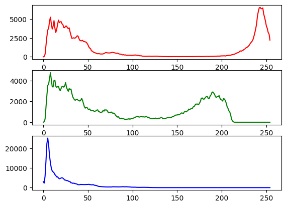
Let’s now get an histogram of colors. When you execute the following code, you will get a single array of values, frequency of each band (R, G, B etc.) concatenated together. In the following code, we will assume that we are working with an image of 3 bands (RGB mode) and each band is represented by 8 bits. We will plot the histogram of different colors.

from PIL import Image
import matplotlib.pyplot as plot

imgfile = Image.open("../images/flower.jpg")
histogram = imgfile.histogram()
# we have three bands (for this image)
red = histogram[0:255]
green = histogram[256:511]
blue = histogram[512:767]
fig, (axis1, axis2, axis3) = plot.subplots(nrows=3, ncols=1)
axis1.plot(red, color="red")
axis2.plot(green, color="green")
axis3.plot(blue, color="blue")
plot.show()

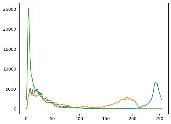
But if you wish to see all of them in one single plot.

from PIL import Image
import matplotlib.pyplot as plot

imgfile = Image.open("../images/flower.jpg")
histogram = imgfile.histogram()
red = histogram[0:255]
green = histogram[256:511]
blue = histogram[512:767]
x = range(255)
y = []
for i in x:
    y.append((red[i], green[i], blue[i]))
plot.plot(x, y)
plot.show()

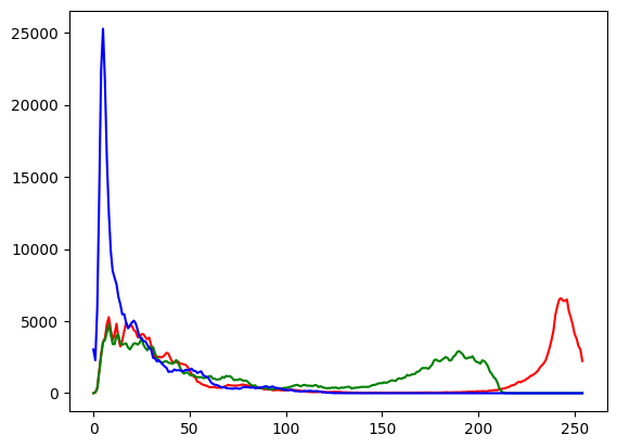
But we do not wish to loose the band colors.

from PIL import Image
import matplotlib.pyplot as plot

imgfile = Image.open("../images/flower.jpg")
histogram = imgfile.histogram()
red = histogram[0:255]
green = histogram[256:511]
blue = histogram[512:767]
x = range(255)
y = []
for i in x:
    y.append((red[i], green[i], blue[i]))
figure, axes = plot.subplots()
axes.set_prop_cycle("color", ["red", "green", "blue"])
plot.plot(x, y)
plot.show()

Your next question is to get the top 20 intensities in each band and create a single plot of these top intensities. Write a python program that can achieve this.

Exercise 3 [★★]

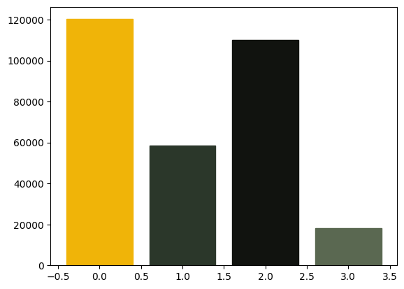
In this exercise, we will take a look at KMeans clustering algorithm. Continuing with images, we will now find 4 predominant colors in an image.

from PIL import Image
import numpy
import math
import matplotlib.pyplot as plot
from sklearn.cluster import KMeans

imgfile = Image.open("../images/flower.jpg")
numarray = numpy.array(imgfile.getdata(), numpy.uint8)
clusters = KMeans(n_clusters=4, n_init=2)
clusters.fit(numarray)
npbins = numpy.arange(0, 5)
histogram = numpy.histogram(clusters.labels_, bins=npbins)
labels = numpy.unique(clusters.labels_)
barlist = plot.bar(labels, histogram[0])
for i in range(4):
    barlist[i].set_color(
        "#%02x%02x%02x"
        % (
            math.ceil(clusters.cluster_centers_[i][0]),
            math.ceil(clusters.cluster_centers_[i][1]),
            math.ceil(clusters.cluster_centers_[i][2]),
        )
    )
plot.show()

For your next question, your goal is to understand the above code and achieve the following:

1. Assume that the number of clusters is given by the user, generalize the above code.

2. In case of bar chart, ensure that the bars are arranged in the descending order of the frequency of colors.

3. Also add support for pie chart in addition to the bar chart. Ensure that we use the image colors as the wedge colors. (e.g., given below)

4. Do you have any interesting observations?

Exercise 4 [★★]

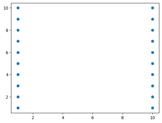
We will try to get more clusters and also check the time taken by each of these algorithms. Let’s start with some very simple exercises to experiment with the KMeans algorithm. Consider the following data and visualize it using a scatter plot.

import numpy as np
import matplotlib.pyplot as plot

numarray = np.array(
    [
        [1, 1],
        [1, 2],
        [1, 3],
        [1, 4],
        [1, 5],
        [1, 6],
        [1, 7],
        [1, 8],
        [1, 9],
        [1, 10],
        [10, 1],
        [10, 2],
        [10, 3],
        [10, 4],
        [10, 5],
        [10, 6],
        [10, 7],
        [10, 8],
        [10, 9],
        [10, 10],
    ]
)

plot.scatter(numarray[:, 0], numarray[:, 1])
plot.show()

Visually, it is quite evident that there are two clusters. But let’s use KMeans algorithm to obtain the 2 clusters. We will first see the labels of our clustered data.

import numpy as np
import matplotlib.pyplot as plot
from sklearn.cluster import KMeans

numarray = np.array(
    [
        [1, 1],
        [1, 2],
        [1, 3],
        [1, 4],
        [1, 5],
        [1, 6],
        [1, 7],
        [1, 8],
        [1, 9],
        [1, 10],
        [10, 1],
        [10, 2],
        [10, 3],
        [10, 4],
        [10, 5],
        [10, 6],
        [10, 7],
        [10, 8],
        [10, 9],
        [10, 10],
    ]
)

clusters = KMeans(n_clusters=2, n_init=2)
clusters.fit(numarray)
print(clusters.labels_)

[1 1 1 1 1 1 1 1 1 1 0 0 0 0 0 0 0 0 0 0]

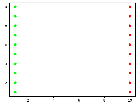
Now, we will visualize the clusters using a scatter plot. We will use two colors for visually distinguishing them.

import numpy as np
import matplotlib.pyplot as plot
from sklearn.cluster import KMeans

numarray = np.array(
    [
        [1, 1],
        [1, 2],
        [1, 3],
        [1, 4],
        [1, 5],
        [1, 6],
        [1, 7],
        [1, 8],
        [1, 9],
        [1, 10],
        [10, 1],
        [10, 2],
        [10, 3],
        [10, 4],
        [10, 5],
        [10, 6],
        [10, 7],
        [10, 8],
        [10, 9],
        [10, 10],
    ]
)

clusters = KMeans(n_clusters=2, n_init=2)
clusters.fit(numarray)
colors = np.array(["#ff0000", "#00ff00"])

plot.scatter(numarray[:, 0], numarray[:, 1], c=colors[clusters.labels_])
plot.show()

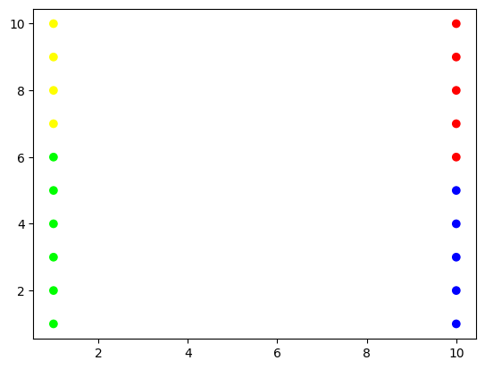
What if we tried to obtain 4 clusters? Try running the following code, multiple times. Any observation? Try changing the value of n_init with higher values.

import numpy as np
import matplotlib.pyplot as plot
from sklearn.cluster import KMeans

numarray = np.array(
    [
        [1, 1],
        [1, 2],
        [1, 3],
        [1, 4],
        [1, 5],
        [1, 6],
        [1, 7],
        [1, 8],
        [1, 9],
        [1, 10],
        [10, 1],
        [10, 2],
        [10, 3],
        [10, 4],
        [10, 5],
        [10, 6],
        [10, 7],
        [10, 8],
        [10, 9],
        [10, 10],
    ]
)

clusters = KMeans(n_clusters=4, n_init=2)
clusters.fit(numarray)
colors = np.array(["#ff0000", "#00ff00", "#0000ff", "#ffff00"])

plot.scatter(numarray[:, 0], numarray[:, 1], c=colors[clusters.labels_])
plot.show()

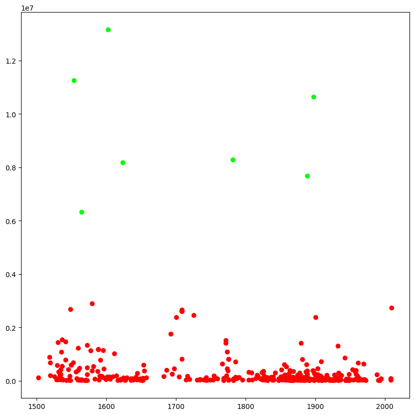
Now we will try obtaining clusters with some real data (reference: citypopulation.json, Source: Wikidata). It contains information concerning different cities of the world: city name, year of its foundation and its population in the year 2010. In the following code, we want to cluster population data and to observe whether there is any correlation between age and recent population (2010) statistics. In the following code, there is a commented line. You can un-comment it to try with different population numbers. Any observation? Why did we use LabelEncoder? What is its purpose?

from pandas import json_normalize
from sklearn.preprocessing import LabelEncoder
import pandas as pd
import json

data = json.load(open("../data/citypopulation.json"))
dataframe = json_normalize(data)
le = LabelEncoder()
dataframe["cityLabel"] = le.fit_transform(dataframe["cityLabel"])
dataframe = dataframe.astype(
    dtype={"year": "<i4", "cityLabel": "<U200", "population": "i"}
)
dataframe = dataframe.loc[dataframe["year"] > 1500]
# dataframe = dataframe.loc[dataframe['population'] < 700000]
yearPopulation = dataframe[["year", "population"]]
clusters = KMeans(n_clusters=2, n_init=1000)
clusters.fit(yearPopulation.values)
colors = np.array(["#ff0000", "#00ff00", "#0000ff", "#ffff00"])

plot.rcParams["figure.figsize"] = [10, 10]
plot.scatter(
    yearPopulation["year"], yearPopulation["population"], c=colors[clusters.labels_]
)
plot.show()

Now let’s continue working with flower.jpg. Let’s start once again with KMeans and try to get clusters of size between 2 and 11.

from PIL import Image
import numpy
import math
import matplotlib.pyplot as plot
from sklearn.cluster import KMeans

imgfile = Image.open("../images/flower.jpg")
numarray = numpy.array(imgfile.getdata(), numpy.uint8)
X = []
Y = []
fig, axes = plot.subplots(nrows=5, ncols=2, figsize=(20, 25))
xaxis = 0
yaxis = 0
for x in range(2, 12):
    cluster_count = x

    clusters = KMeans(n_clusters=cluster_count, n_init=2)
    clusters.fit(numarray)

    npbins = numpy.arange(0, cluster_count + 1)
    histogram = numpy.histogram(clusters.labels_, bins=npbins)
    labels = numpy.unique(clusters.labels_)
    barlist = axes[xaxis, yaxis].bar(labels, histogram[0])
    if yaxis == 0:
        yaxis = 1
    else:
        xaxis = xaxis + 1
        yaxis = 0
    for i in range(cluster_count):
        barlist[i].set_color(
            "#%02x%02x%02x"
            % (
                math.ceil(clusters.cluster_centers_[i][0]),
                math.ceil(clusters.cluster_centers_[i][1]),
                math.ceil(clusters.cluster_centers_[i][2]),
            )
        )
plot.show()

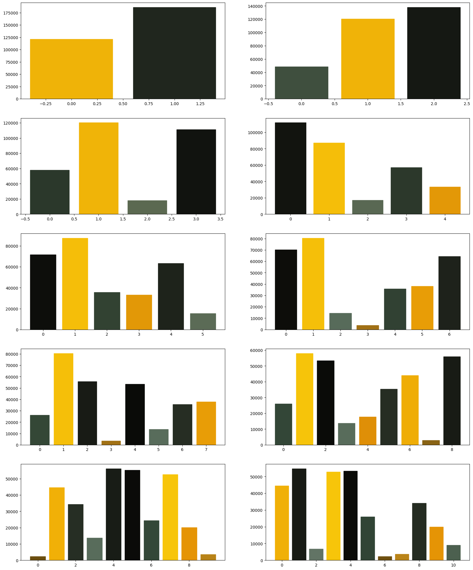
Your next goal is to test the above code for cluster sizes between 2 and 21 which will give you the figure given below.

Note: The following image was generated after 6 minutes. Optionally, you can add print statements to test whether your code is working fine.

Now we modify the above algorithm to use MiniBatchKMeans clustering algorithm (refer here). Observe the changes.

from PIL import Image
import numpy
import math
import matplotlib.pyplot as plot
from sklearn.cluster import MiniBatchKMeans

imgfile = Image.open("../images/flower.jpg")
numarray = numpy.array(imgfile.getdata(), numpy.uint8)
X = []
Y = []
fig, axes = plot.subplots(nrows=5, ncols=2, figsize=(20, 25))
xaxis = 0
yaxis = 0
for x in range(2, 12):
    cluster_count = x

    clusters = MiniBatchKMeans(n_clusters=cluster_count, n_init=2)
    clusters.fit(numarray)

    npbins = numpy.arange(0, cluster_count + 1)
    histogram = numpy.histogram(clusters.labels_, bins=npbins)
    labels = numpy.unique(clusters.labels_)
    barlist = axes[xaxis, yaxis].bar(labels, histogram[0])
    if yaxis == 0:
        yaxis = 1
    else:
        xaxis = xaxis + 1
        yaxis = 0
    for i in range(cluster_count):
        barlist[i].set_color(
            "#%02x%02x%02x"
            % (
                math.ceil(clusters.cluster_centers_[i][0]),
                math.ceil(clusters.cluster_centers_[i][1]),
                math.ceil(clusters.cluster_centers_[i][2]),
            )
        )
plot.show()

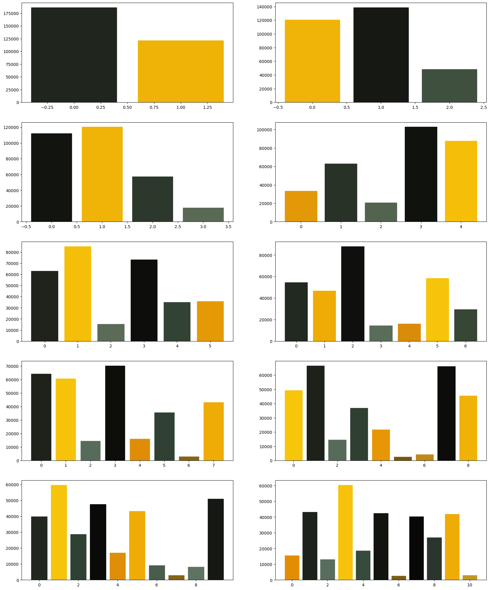
What did you observe? Your next goal is to test the above code for cluster sizes between 2 and 21 which will give you the figure given below. What are your conclusions? In order to compare the two algorithms, we consider the time taken by each of these algorithms. We will repeat the above experiment, but this time we will plot the time taken to obtain clusters of different sizes. We start with KMeans.

from PIL import Image
import numpy
import math
import time
import matplotlib.pyplot as plot
from sklearn.cluster import KMeans

imgfile = Image.open("../images/flower.jpg")
numarray = numpy.array(imgfile.getdata(), numpy.uint8)
X = []
Y = []
for x in range(1, 20):
    cluster_count = x

    start_time = time.time()
    clusters = KMeans(n_clusters=cluster_count, n_init=2)
    clusters.fit(numarray)
    end_time = time.time()
    total_time = end_time - start_time
    print("Total time: ", x, ":", total_time)
    X.append(x)
    Y.append(total_time)
plot.bar(X, Y)
plot.show()

Total time:  1 : 0.2527611255645752
Total time:  2 : 0.1887354850769043

Total time:  3 : 0.2924156188964844

Total time:  4 : 0.29050135612487793

Total time:  5 : 0.313143253326416

Total time:  6 : 0.31256961822509766

Total time:  7 : 0.4131293296813965

Total time:  8 : 0.4218709468841553

Total time:  9 : 0.5578181743621826

Total time:  10 : 0.4680898189544678

Total time:  11 : 0.43189382553100586

Total time:  12 : 0.4564704895019531

Total time:  13 : 0.5062034130096436

Total time:  14 : 0.4742591381072998

Total time:  15 : 0.5103898048400879

Total time:  16 : 0.5378174781799316

Total time:  17 : 0.5601310729980469

Total time:  18 : 0.9107832908630371

Total time:  19 : 0.7426881790161133

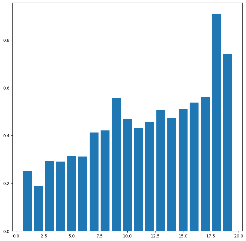
You may get a graph similar to the following.

We now use MiniBatchKMeans.

from PIL import Image
import numpy
import math
import time
import matplotlib.pyplot as plot
from sklearn.cluster import MiniBatchKMeans

imgfile = Image.open("../images/flower.jpg")
numarray = numpy.array(imgfile.getdata(), numpy.uint8)
X = []
Y = []
for x in range(1, 20):
    cluster_count = x

    start_time = time.time()
    clusters = MiniBatchKMeans(n_clusters=cluster_count, n_init=2)
    clusters.fit(numarray)
    end_time = time.time()
    total_time = end_time - start_time
    print("Total time: ", x, ":", total_time)
    X.append(x)
    Y.append(total_time)
plot.bar(X, Y)
plot.show()

Total time:  1 : 0.009935379028320312
Total time:  2 : 0.010888338088989258
Total time:  3 : 0.026899099349975586
Total time:  4 : 0.01895594596862793
Total time:  5 : 0.04577207565307617
Total time:  6 : 0.0156857967376709
Total time:  7 : 0.025664806365966797

Total time:  8 : 0.0608363151550293
Total time:  9 : 0.045433759689331055
Total time:  10 : 0.01137542724609375
Total time:  11 : 0.05837202072143555
Total time:  12 : 0.05266308784484863

Total time:  13 : 0.05564141273498535
Total time:  14 : 0.050501108169555664
Total time:  15 : 0.020290374755859375
Total time:  16 : 0.015059709548950195
Total time:  17 : 0.05481863021850586

Total time:  18 : 0.07881879806518555
Total time:  19 : 0.024054527282714844

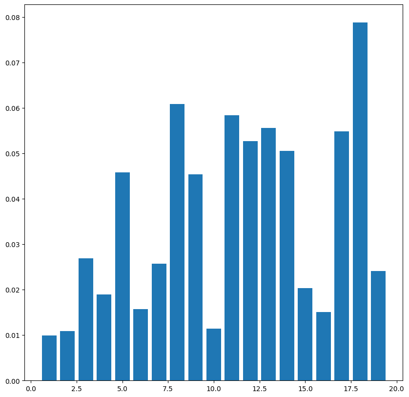
You may get a graph similar to the following.

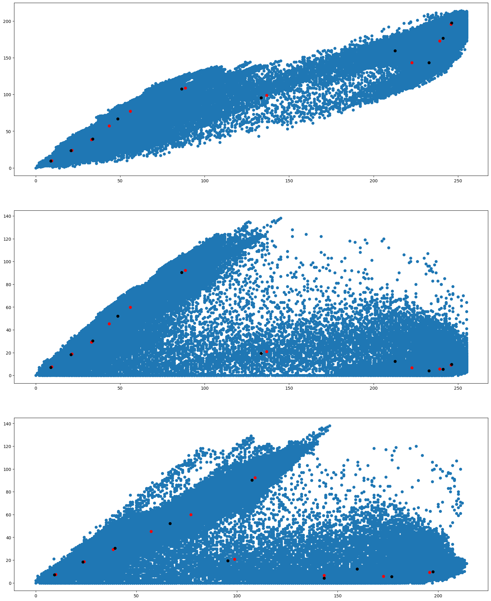
Now test the above code using MiniBatchKMeans algorithm with cluster sizes between 2 and 50. What are your observations? Finally we want to see whether we get the same cluster centers from both the algorithms. Run the following program to see the cluster centers produced by the two algorithms. We use two different colors (red and black) to distinguish the cluster centers from the two algorithms.

from PIL import Image
import numpy
import math
import matplotlib.pyplot as plot
from sklearn.cluster import KMeans
from sklearn.cluster import MiniBatchKMeans

imgfile = Image.open("../images/flower.jpg")
numarray = numpy.array(imgfile.getdata(), numpy.uint8)

cluster_count = 10

clusters = KMeans(n_clusters=cluster_count, n_init=2)
clusters.fit(numarray)

mclusters = MiniBatchKMeans(n_clusters=cluster_count, n_init=2)
mclusters.fit(numarray)

fig, axes = plot.subplots(nrows=3, ncols=1, figsize=(20, 25))
# Scatter plot for RG (RGB)
axes[0].scatter(numarray[:, 0], numarray[:, 1])
axes[0].scatter(
    clusters.cluster_centers_[:, 0], clusters.cluster_centers_[:, 1], c="red"
)
axes[0].scatter(
    mclusters.cluster_centers_[:, 0], mclusters.cluster_centers_[:, 1], c="black"
)

# Scatter plot of RB (RGB)
axes[1].scatter(numarray[:, 0], numarray[:, 2])
axes[1].scatter(
    clusters.cluster_centers_[:, 0], clusters.cluster_centers_[:, 2], c="red"
)
axes[1].scatter(
    mclusters.cluster_centers_[:, 0], mclusters.cluster_centers_[:, 2], c="black"
)

# Scatter plot of GB (RGB)
axes[2].scatter(numarray[:, 1], numarray[:, 2])
axes[2].scatter(
    clusters.cluster_centers_[:, 1], clusters.cluster_centers_[:, 2], c="red"
)
axes[2].scatter(
    mclusters.cluster_centers_[:, 1], mclusters.cluster_centers_[:, 2], c="black"
)

<matplotlib.collections.PathCollection at 0x7f70156c7520>

We would like to see how the individual pixel values have been clustered. Run the following program a couple of times.

from PIL import Image
import numpy
import math
import time
import matplotlib.pyplot as plot
from sklearn.cluster import KMeans
from sklearn.cluster import MiniBatchKMeans

imgfile = Image.open("../images/flower.jpg")
numarray = numpy.array(imgfile.getdata(), numpy.uint8)

cluster_count = 10

mclusters = MiniBatchKMeans(n_clusters=cluster_count, n_init=2)
mclusters.fit(numarray)

npbins = numpy.arange(0, cluster_count + 1)
histogram = numpy.histogram(mclusters.labels_, bins=npbins)
labels = numpy.unique(mclusters.labels_)

fig, axes = plot.subplots(nrows=3, ncols=2, figsize=(20, 25))

# Scatter plot for RG (RGB)
colors = []
for i in range(len(numarray)):
    j = mclusters.labels_[i]
    colors.append(
        "#%02x%02x%02x"
        % (
            math.ceil(mclusters.cluster_centers_[j][0]),
            math.ceil(mclusters.cluster_centers_[j][1]),
            0,
        )
    )

axes[0, 0].scatter(numarray[:, 0], numarray[:, 1], c=colors)
axes[0, 0].scatter(
    mclusters.cluster_centers_[:, 0],
    mclusters.cluster_centers_[:, 1],
    marker="+",
    c="red",
)

# Scatter plot for RB (RGB)
colors = []
for i in range(len(numarray)):
    j = mclusters.labels_[i]
    colors.append(
        "#%02x%02x%02x"
        % (
            math.ceil(mclusters.cluster_centers_[j][0]),
            0,
            math.ceil(mclusters.cluster_centers_[j][2]),
        )
    )

axes[1, 0].scatter(numarray[:, 0], numarray[:, 2], c=colors)
axes[1, 0].scatter(
    mclusters.cluster_centers_[:, 0],
    mclusters.cluster_centers_[:, 2],
    marker="+",
    c="white",
)

# Scatter plot for GB (RGB)
colors = []
for i in range(len(numarray)):
    j = mclusters.labels_[i]
    colors.append(
        "#%02x%02x%02x"
        % (
            0,
            math.ceil(mclusters.cluster_centers_[j][1]),
            math.ceil(mclusters.cluster_centers_[j][2]),
        )
    )

axes[2, 0].scatter(numarray[:, 1], numarray[:, 2], c=colors)
axes[2, 0].scatter(
    mclusters.cluster_centers_[:, 1],
    mclusters.cluster_centers_[:, 2],
    marker="+",
    c="yellow",
)

clusters = KMeans(n_clusters=cluster_count, n_init=2)
clusters.fit(numarray)

npbins = numpy.arange(0, cluster_count + 1)
histogram = numpy.histogram(clusters.labels_, bins=npbins)
labels = numpy.unique(clusters.labels_)

# Scatter plot for RG (RGB)
colors = []
for i in range(len(numarray)):
    j = clusters.labels_[i]
    colors.append(
        "#%02x%02x%02x"
        % (
            math.ceil(clusters.cluster_centers_[j][0]),
            math.ceil(clusters.cluster_centers_[j][1]),
            0,
        )
    )

axes[0, 1].scatter(numarray[:, 0], numarray[:, 1], c=colors)
axes[0, 1].scatter(
    clusters.cluster_centers_[:, 0],
    clusters.cluster_centers_[:, 1],
    marker="+",
    c="red",
)

# Scatter plot for RB (RGB)
colors = []
for i in range(len(numarray)):
    j = clusters.labels_[i]
    colors.append(
        "#%02x%02x%02x"
        % (
            math.ceil(clusters.cluster_centers_[j][0]),
            0,
            math.ceil(clusters.cluster_centers_[j][2]),
        )
    )

axes[1, 1].scatter(numarray[:, 0], numarray[:, 2], c=colors)
axes[1, 1].scatter(
    clusters.cluster_centers_[:, 0],
    clusters.cluster_centers_[:, 2],
    marker="+",
    c="white",
)

# Scatter plot for GB (RGB)
colors = []
for i in range(len(numarray)):
    j = clusters.labels_[i]
    colors.append(
        "#%02x%02x%02x"
        % (
            0,
            math.ceil(clusters.cluster_centers_[j][1]),
            math.ceil(clusters.cluster_centers_[j][2]),
        )
    )

axes[2, 1].scatter(numarray[:, 1], numarray[:, 2], c=colors)
axes[2, 1].scatter(
    clusters.cluster_centers_[:, 1],
    clusters.cluster_centers_[:, 2],
    marker="+",
    c="yellow",
)
plot.show()

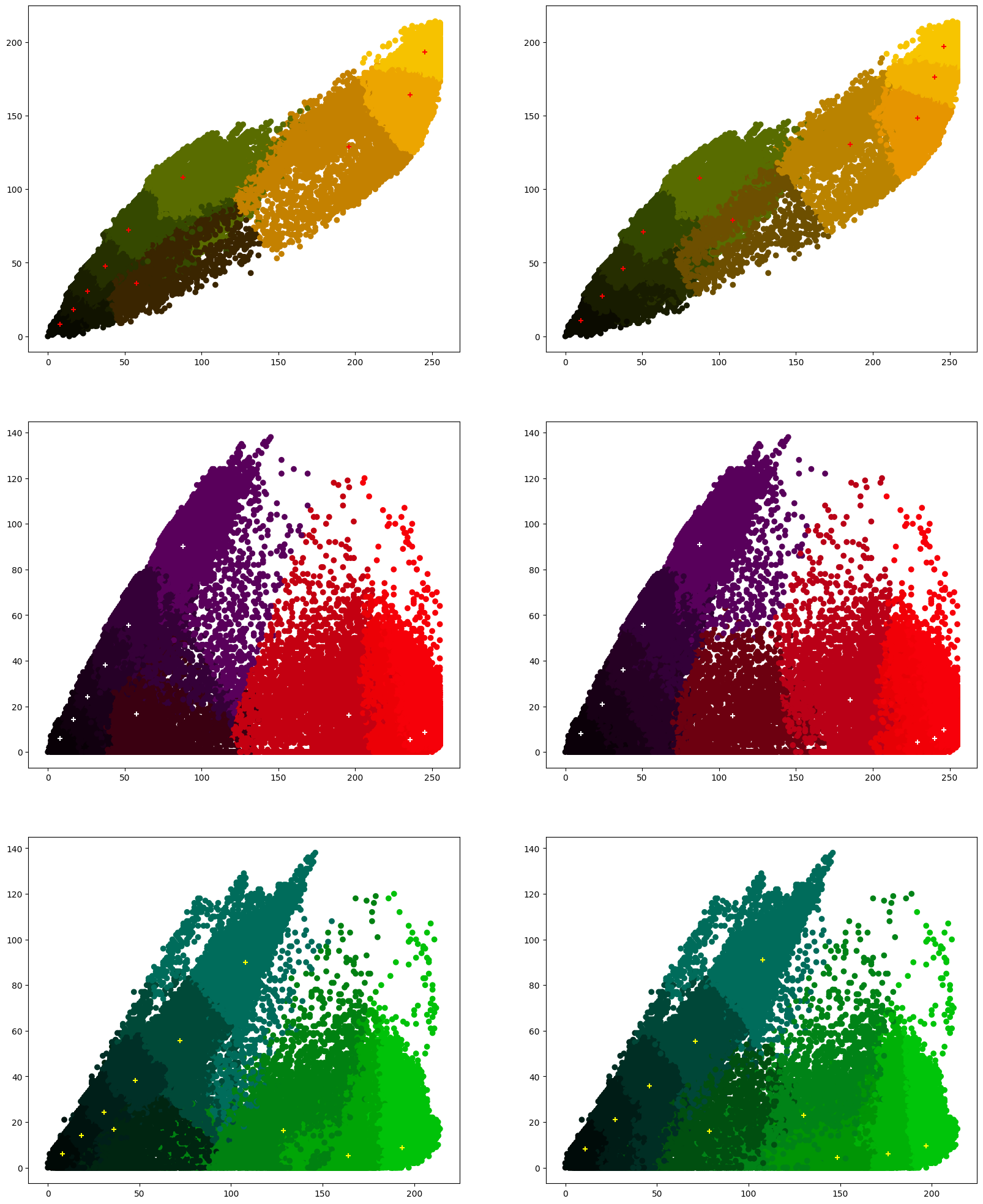
What are your conclusions?

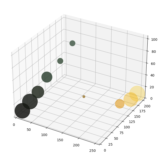
Exercise 5

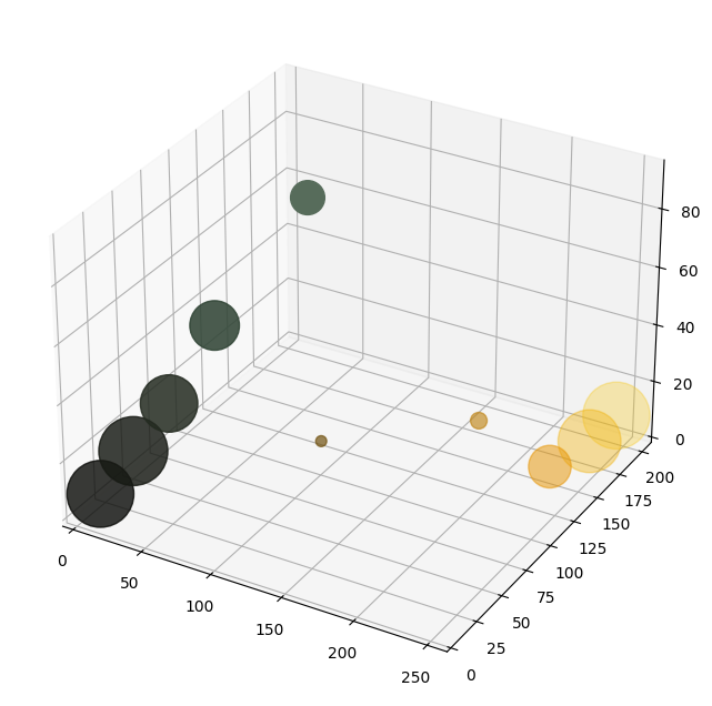
Finally, we plot these clusters in 3D. Test the following graph with different images and different numbers of clusters.

from PIL import Image
import numpy
import math
import matplotlib.pyplot as plot
from sklearn.cluster import KMeans
from sklearn.cluster import MiniBatchKMeans
from sklearn.preprocessing import scale, minmax_scale

cluster_count = 10

imgfile = Image.open("../images/flower.jpg")
numarray = numpy.array(imgfile.getdata(), numpy.uint8)

# Calculating the clusters
clusters = KMeans(n_clusters=cluster_count, n_init=2)
clusters.fit(numarray)


# Calculating the number of pixels belonging to each cluster
unique, frequency = numpy.unique(clusters.labels_, return_counts=True)

# Scaling the frequency value between 50 and 2000 (these values were randomly chosen)
scaled_frequency = minmax_scale(frequency, feature_range=(50, 2000))

colors = []
for i in range(len(clusters.cluster_centers_)):
    colors.append(
        "#%02x%02x%02x"
        % (
            math.ceil(clusters.cluster_centers_[i][0]),
            math.ceil(clusters.cluster_centers_[i][1]),
            math.ceil(clusters.cluster_centers_[i][2]),
        )
    )

# 3D scatter plot
plot.figure(figsize=(8, 8))
axes = plot.axes(projection="3d")
axes.scatter3D(
    clusters.cluster_centers_[:, 0],
    clusters.cluster_centers_[:, 1],
    clusters.cluster_centers_[:, 2],
    c=colors,
    s=scaled_frequency,
);

Compare the two approaches (MiniBatchKMeans vs. KMeans)?

from PIL import Image
import numpy
import math
import matplotlib.pyplot as plot
from sklearn.cluster import KMeans
from sklearn.cluster import MiniBatchKMeans
from sklearn.preprocessing import scale, minmax_scale

cluster_count = 10

imgfile = Image.open("../images/flower.jpg")
numarray = numpy.array(imgfile.getdata(), numpy.uint8)

# Calculating the clusters
clusters = MiniBatchKMeans(n_clusters=cluster_count, n_init=2)
clusters.fit(numarray)


# Calculating the number of pixels belonging to each cluster
unique, frequency = numpy.unique(clusters.labels_, return_counts=True)

# Scaling the frequency value between 50 and 2000 (these values were randomly chosen)
scaled_frequency = minmax_scale(frequency, feature_range=(50, 2000))

colors = []
for i in range(len(clusters.cluster_centers_)):
    colors.append(
        "#%02x%02x%02x"
        % (
            math.ceil(clusters.cluster_centers_[i][0]),
            math.ceil(clusters.cluster_centers_[i][1]),
            math.ceil(clusters.cluster_centers_[i][2]),
        )
    )

# 3D scatter plot
plot.figure(figsize=(8, 8))
axes = plot.axes(projection="3d")
axes.scatter3D(
    clusters.cluster_centers_[:, 0],
    clusters.cluster_centers_[:, 1],
    clusters.cluster_centers_[:, 2],
    c=colors,
    s=scaled_frequency,
);