
Goals
- Understanding the translation pattern
Exercise 1.1
Download
Download the data from https://zenodo.org/record/3271358.
View the data contents. As you can see in the output, there are four columns: timestamp, property, language and type.
Taking an example line from this dataset,
2013-09-10T22:43:54Z,P856,en,label
corresponds to the action that an English label of Property P856 was added for the first time at 2013-09-10T22:43:54Z.
Following is a description of each column.
- timestamp: the time at which an action was made. For example, 2013-09-10T22:43:54Z
- property: Wikidata property identifier. It uses the P-number, For example, P856
- language: the language in which a label/description/alias was first translated
- type: It could be one of the following values: label, description and alias
Creation of dataframe
              import pandas as pd

              dataframe = pd.read_csv("multilingual_wikidata_translation_flow.csv")
              # remove duplicates
              dataframe = dataframe.drop_duplicates()

              # remove rows with missing values
              dataframe = dataframe.dropna()
              print(dataframe)
Get a detailed information of the given dataframe.
dataframe.describe()
Let us now take a look at the translation of labels in different languages for a given property.
dataframe.loc[(dataframe["property"]=="P856") & (dataframe["type"]=="label")]
We will check the data available for a property like P856.
            ptranslation = dataframe.loc[(dataframe["property"]=="P856")]
            print(ptranslation)
You can also add additional conditions to filter out any information. The code below filters out the translation of labels of property P856. Please copy the code below and create new cells for testing with different properties and see the results for translation of descriptions and aliases. What are your first observations? Please note them as comments in your notebook.
            ptranslation = dataframe.loc[(dataframe["property"]=="P856") & (dataframe["type"]=="label")]
            print(ptranslation)
Visualization of translation
Our next goal is to plot the translation of a property and see whether we can observe any translation pattern. Please copy the code below and create new cells for testing with different properties and plot the results. In this plot, we plot the time on the x-axis and translation type on the y-axis.
import matplotlib
import  matplotlib.pyplot as plot
from  dateutil import parser
import  numpy as np

ptranslation  = dataframe.loc[(dataframe["property"]=="P856")]

x  = []
y  = []
z  = []
for  i in range(0, len(ptranslation['timestamp'])):
   #parsing the date in string and converting it to datetime
   try:
       value = parser.parse(ptranslation['timestamp'].iloc[i])
       x.append(value)
   except Exception:
       continue
   y.append(ptranslation['type'].iloc[i])
   z.append(ptranslation['language'].iloc[i])

#creating  a plot
plot.rcParams["figure.figsize"]  = (25, 9)

colors  = matplotlib.cm.rainbow(np.linspace(0, 1, 3))
tcolors  = {'label': colors[0],
     'description':colors[1],
     'alias':colors[2]
    }
cs  = [tcolors[i] for i in y]
fig,  ax = plot.subplots()
ax.scatter(x, y, s=30, color=cs)

plot.xlabel("Time")
plot.ylabel("Translation type")

#annotating  the points
for i, txt in enumerate(z):
  ax.annotate(txt, (x[i], y[i]))

fig.show()
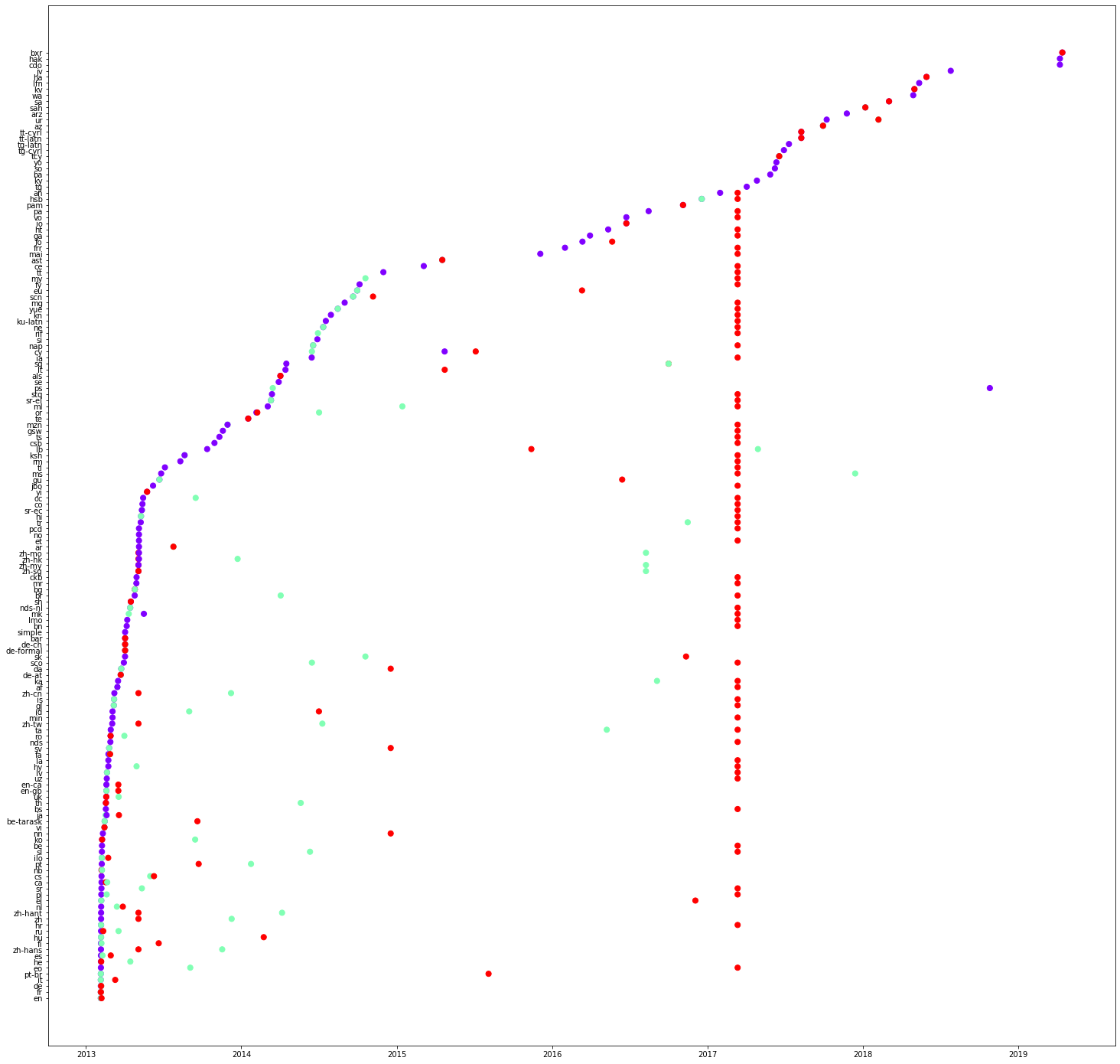
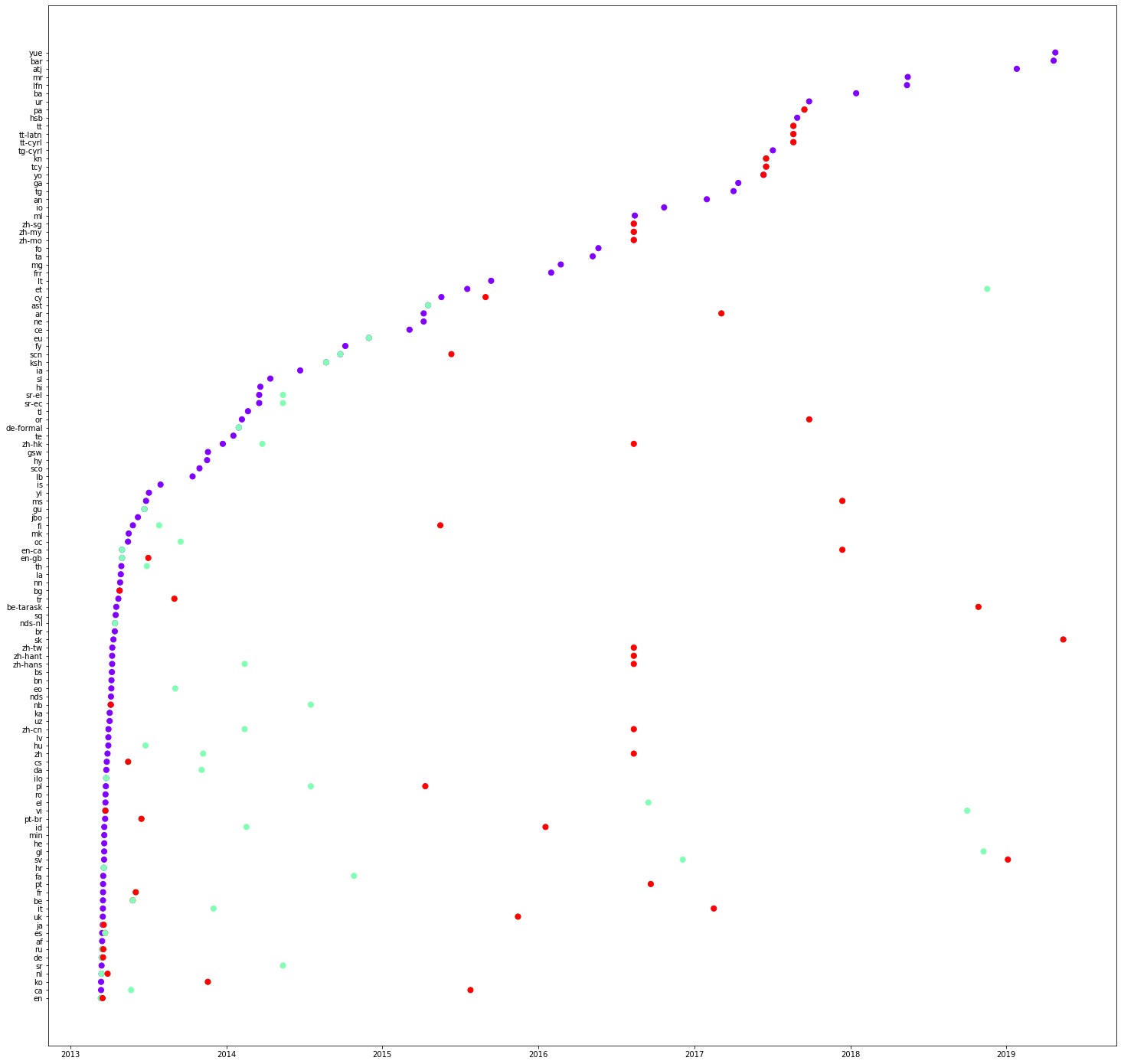
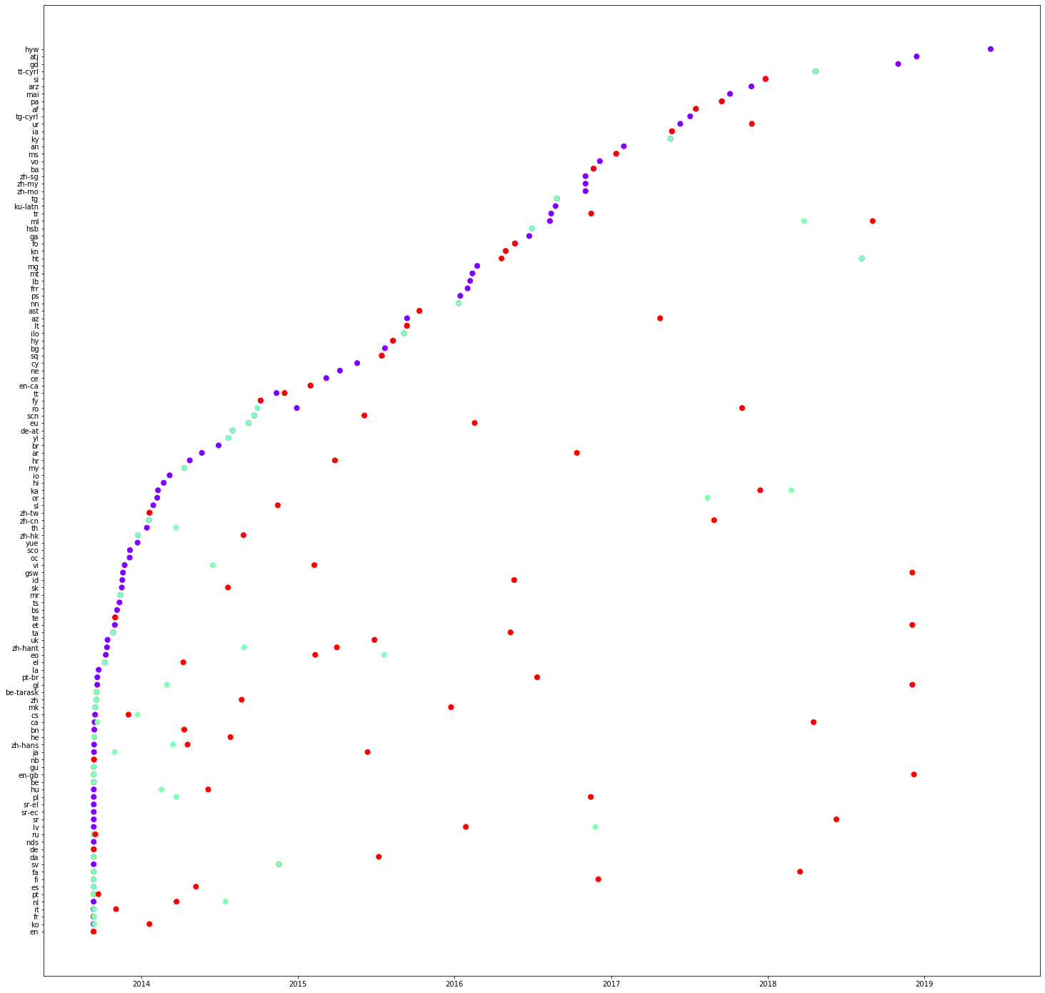
Now, we plot another graph, this time, language on the y-axis and time on the x-axis.
import matplotlib
import matplotlib.pyplot as plot
from dateutil import parser
import numpy as np

ptranslation = dataframe.loc[(dataframe["property"]=="P279")]

x = []
y = []
z = []
for i in range(0, len(ptranslation['timestamp'])):
   try:
     #parsing the date in string and converting it to datetime
    value = parser.parse(ptranslation['timestamp'].iloc[i])
    x.append(value)
   except Exception:
       continue
   y.append(ptranslation['type'].iloc[i])
   z.append(ptranslation['language'].iloc[i])

#creating a plot
colors = matplotlib.cm.rainbow(np.linspace(0, 1, 3))
tcolors = {'label': colors[0],
              'description':colors[1],
              'alias':colors[2]
           }
cs = [tcolors[i] for i in y]

plot.rcParams["figure.figsize"] = (25, 25)
fig, ax = plot.subplots()
ax.scatter(x, z, s=50, color=cs)


plot.xlabel("Time")
plot.ylabel("Language")

# saving the plot in a file
plot.savefig('translation.png')
fig.show()
Following are three plots concerning properties: P31, P279 and P856 respectively. What are your observations on the values on the y-axis? Please note them as comments on the notebook. You can also see that some translations can be even made in a single edit. Please check a column of red lines in the first figure (P31).
In the code given below, we select some languages and see the order of translation. Copy the code below and plot the graphs for different properties. Please note your observations as comments on the notebook.
import matplotlib
import matplotlib.pyplot as plot
from dateutil import parser
import numpy as np

#list of languages under consideration
langlist  = ["fr", "es", "en", "de", "it", "pt", "ja"]
ptranslation  = dataframe.loc[(dataframe["property"]=="P18") & (dataframe["language"].isin (langlist))]
print(ptranslation)

x= []
y= []
z= []
for i in range(0, len(ptranslation['timestamp'])):
   try:
       #parsing the date in string and converting it to datetime
      value = parser.parse(ptranslation['timestamp'].iloc[i])
    x.append(value)
   except Exception:
       continue
   y.append(ptranslation['type'].iloc[i])
   z.append(ptranslation['language'].iloc[i])

#creating  a plot
colors  = matplotlib.cm.rainbow(np.linspace(0, 1, 3))
tcolors  = {'label': colors[0],
              'description':colors[1],
              'alias':colors[2]
            }
cs  = [tcolors[i] for i in y]

plot.rcParams["figure.figsize"]  = (10, 5)
fig,  ax = plot.subplots()
ax.scatter(x,  z, s=50, color=cs)

plot.savefig('translation.png')
fig.show()
Exercise 1.2
We used plotting techniques to manually detect some patterns of translation. Now we use other algorithms to see whether groups of languages are always present together
Before continuing, we need to install the library mlxtend.
!pip install mlxtend
Next we prepare the language dataset. We will focus on the translation of property labels. We create a list of list of available translations of labels of all the properties from our dataset
#prepare dataset of languages
languageorder = []
labeldataframe = dataframe.loc[(dataframe["type"] == "label")]
groups = labeldataframe.groupby(["property"])
for k, group in groups:
  languageorder.append(list(groups.get_group((k))["language"]))
print(languageorder);
This will give us the following output.
[['en', 'it', 'fi', 'fr', 'de', 'zh-hans', 'ru', 'hu', 'he', 'nl', 'pt', 'pl', 'ca', 'cs', 'ilo', 'zh', 'nb', 'ko',..
Now we calculate the frequent itemsets using apriori algorithm. Please uncomment the print statement to see the intermediate dataframe.
from mlxtend.preprocessing import TransactionEncoder
from mlxtend.frequent_patterns import apriori

te = TransactionEncoder()

te_ary = te.fit(languageorder).transform(languageorder)

# preparation of data frame
df = pd.DataFrame(te_ary, columns=te.columns_)
#print(df)

#use of apriori algorithm
frequent_itemsets = apriori(df, min_support=0.75, use_colnames=True)

print (frequent_itemsets)
The program uses a minimum support of 0.75. We see that English labels are present for all the properties, whereas French labels are only available for 93% of the properties. On considering pairs of languages, we see that English and Arabic are present in 93% of the translations. As we go further below, we see combinations of 3, 4, 5 languages etc.
Please change this value between 0 and 1 and see the output.
| S.No. | support | itemsets | |
|---|---|---|---|
| 0 | 0.998424 | (ar) | |
| 1 | 0.759414 | (ca) | |
| 2 | 1.000000 | (en) | |
| 3 | 0.932409 | (fr) | |
| 4 | 0.993540 | (nl) | |
| 5 | 0.985978 | (uk) | |
| 6 | 0.758626 | (ar, ca) | |
| 7 | 0.998424 | (en, ar) | |
| 8 | 0.931621 | (ar, fr) | |
| 9 | 0.992752 | (nl, ar) | |
| 10 | 0.985663 | (ar, uk) | |
| 11 | 0.759414 | (en, ca) | |
| 12 | 0.759256 | (nl, ca) | |
| 13 | 0.754215 | (uk, ca) | |
| 14 | 0.932409 | (en, fr) | |
| 15 | 0.993540 | (nl, en) | |
| 16 | 0.985978 | (en, uk) | |
| 17 | 0.931779 | (nl, fr) | |
| 18 | 0.928155 | (uk, fr) | |
| 19 | 0.985663 | (nl, uk) | |
| 20 | 0.758626 | (en, ar, ca) | |
| 21 | 0.758469 | (nl, ar, ca) | |
| 22 | 0.753899 | (ar, uk, ca) | |
| 23 | 0.931621 | (en, ar, fr) | |
| 24 | 0.992752 | (nl, en, ar) | |
| 25 | 0.985663 | (en, ar, uk) | |
| 26 | 0.931149 | (nl, ar, fr) | |
| 27 | 0.927997 | (ar, uk, fr) | |
| 28 | 0.985347 | (nl, ar, uk) | |
| 29 | 0.759256 | (nl, en, ca) | |
| 30 | 0.754215 | (en, uk, ca) | |
| 31 | 0.754057 | (nl, uk, ca) | |
| 32 | 0.931779 | (nl, en, fr) | |
| 33 | 0.928155 | (en, uk, fr) | |
| 34 | 0.985663 | (nl, en, uk) | |
| 35 | 0.927840 | (nl, uk, fr) | |
| 36 | 0.758469 | (nl, en, ar, ca) | |
| 37 | 0.753899 | (en, ar, uk, ca) | |
| 38 | 0.753742 | (nl, ar, uk, ca) | |
| 39 | 0.931149 | (nl, en, ar, fr) | |
| 40 | 0.927997 | (en, ar, uk, fr) | |
| 41 | 0.985347 | (nl, en, ar, uk) | |
| 42 | 0.927682 | (nl, ar, uk, fr) | |
| 43 | 0.754057 | (nl, en, uk, ca) | |
| 44 | 0.927840 | (nl, en, uk, fr) | |
| 45 | 0.753742 | (ar, en, ca, nl, uk) | |
| 46 | 0.927682 | (ar, en, fr, nl, uk) |
Repeat the above experiment for descriptions and aliases. What are your observations. Please note them in the notebook as comments.
Exercise 1.3
Our next goal is to generate the association rules, i.e, rules of the form. A -> C, where A is the antecedent and C is the consequent.
from mlxtend.frequent_patterns import association_rules

association_rules(frequent_itemsets, metric="confidence", min_threshold=0.95)
It will give us the following output.
| S.No. | antecedents | consequents | antecedent support | consequent support | support | confidence | lift | leverage | conviction |
|---|---|---|---|---|---|---|---|---|---|
| 0 | (de) | (en) | 0.479193 | 0.988966 | 0.477932 | 0.997368 | 1.008496 | 0.004026 | 4.192938 |
| 1 | (de) | (uk) | 0.479193 | 0.960277 | 0.468789 | 0.978289 | 1.018757 | 0.008631 | 1.829646 |
| 2 | (es) | (en) | 0.389975 | 0.988966 | 0.388556 | 0.996362 | 1.007479 | 0.002884 | 3.033137 |
| 3 | (fr) | (en) | 0.713272 | 0.988966 | 0.708859 | 0.993812 | 1.004900 | 0.003457 | 1.783181 |
| 4 | (it) | (en) | 0.413934 | 0.988966 | 0.413146 | 0.998096 | 1.009232 | 0.003779 | 5.795082 |
| 5 | (ru) | (en) | 0.301387 | 0.988966 | 0.300441 | 0.996862 | 1.007984 | 0.002380 | 3.516183 |
| 6 | (en) | (uk) | 0.988966 | 0.960277 | 0.950189 | 0.960791 | 1.000534 | 0.000507 | 1.013087 |
| 7 | (uk) | (en) | 0.960277 | 0.988966 | 0.950189 | 0.989494 | 1.000534 | 0.000507 | 1.050303 |
| 8 | (es) | (uk) | 0.389975 | 0.960277 | 0.383039 | 0.982215 | 1.022845 | 0.008555 | 2.233492 |
| 9 | (fr) | (uk) | 0.713272 | 0.960277 | 0.689470 | 0.966630 | 1.006615 | 0.004531 | 1.190362 |
| 10 | (it) | (uk) | 0.413934 | 0.960277 | 0.405738 | 0.980198 | 1.020745 | 0.008246 | 2.005990 |
| 11 | (ru) | (uk) | 0.301387 | 0.960277 | 0.300126 | 0.995816 | 1.037009 | 0.010711 | 9.493695 |
| 12 | (de, fr) | (en) | 0.391393 | 0.988966 | 0.391078 | 0.999195 | 1.010343 | 0.004003 | 13.698770 |
| 13 | (de, uk) | (en) | 0.468789 | 0.988966 | 0.467686 | 0.997646 | 1.008777 | 0.004069 | 4.687894 |
Let's take a look at one of the association rule (de, fr)->(en). The confidence score is 0.999195. But this rule states that when we have French and German translations available, we will also have the English translation.
You can change the metric to 'lift' and test.
We will now add two columns that will contain the length of antecedents and consequents. As you may have noticed, association rules are dataframes. So we can easily write filter conditions to get antecedents and consequents of length more than 1.
from mlxtend.frequent_patterns import association_rules

arules = association_rules(frequent_itemsets, metric="confidence", min_threshold=0.95)
arules["antecedent_len"] = arules["antecedents"].apply(lambda x: len(x))
arules["consequent_len"] = arules["consequents"].apply(lambda x: len(x))

arules.loc[(arules["antecedent_len"]>1) &
                 (arules["consequent_len"]>1)]
| S.No. | antecedents | consequents | antecedent support | consequent support | support | confidence | lift | leverage | conviction | antecedent_len | consequent_len |
|---|---|---|---|---|---|---|---|---|---|---|---|
| 32 | (de, fr) | (en, uk) | 0.391393 | 0.950189 | 0.383670 | 0.980266 | 1.031653 | 0.011772 | 2.524088 | 2 | 2 |
| 35 | (fr, es) | (en, uk) | 0.332755 | 0.950189 | 0.326765 | 0.981999 | 1.033477 | 0.010585 | 2.767124 | 2 | 2 |
| 38 | (fr, it) | (en, uk) | 0.345523 | 0.950189 | 0.338430 | 0.979471 | 1.030817 | 0.010117 | 2.426342 | 2 | 2 |
Repeat the above experiment for translation of descriptions and aliases. Please note down your observations as comments in your notebook.
Exercise 1.4
Our next goal is to visualize the flow of translation. For this purpose, we install holoviews and bokeh.
!pip install holoviews bokeh --upgrade
First, we create groups for different translations.
languageorder = []
labeldataframe = dataframe.loc[(dataframe["type"] == "label")]
groups = labeldataframe.groupby(["property"])
for k, group in groups:
    languageorder.append(list(groups.get_group((k))["language"]))

languagepairs = []
for lo in languageorder:
    for i in range(0, len(lo)-1):
       languagepairs.append([lo[i], lo[i+1], 1])

lpdataframe = pd.DataFrame(languagepairs)
lpdataframe.columns = ['source', 'target', 'count']

groups = lpdataframe.groupby(["source","target"]).count().reset_index()
print(groups)
Next we visualize them using circular layout. Note the code below, we have only taken 500 combinations of language pairs.
import networkx as nx
import matplotlib.pyplot as plot

G = nx.from_pandas_edgelist(groups[:500], 'source', 'target')

plot.rcParams["figure.figsize"] = (15,15)
pos = nx.circular_layout(G)
nx.draw(G, pos, with_labels=True)
Copy the above code and check the flow of translations for any languages of your choice (number of languages > 20).
Use Bokeh/Holoviews chord layout for visualizing the weights as well.
Exercise 1.5
Prediction
Our final goal is to predict the next language(s) that will be translated, given a sequence of available translations.
Take for example, let's assume we have seen the following sequences of translation.
             [['en', 'it', 'fi', 'fr', 'de', 'nl', 'pt', 'pl', 'ca', 'cs']
               ['en', 'it', 'fi', 'fr', 'de', 'ilo', 'zh', 'nb']
               ['ru', 'hu', 'he', 'nl', 'pt', 'pl', 'ca', 'cs'],
               ...
             ]
Once your model has been trained using this data, it may be able to predict the next possible translation(s).
Example 1: If the user enters the following sequence,
['pt']
your model may return the following language
['pl']
Example 2: If the user enters the following sequence,
['it', 'fi']
your model may return the following language
['fr']
Example 3: If the user enters the following sequence,
['nl', 'pt', 'pl']
your model may return the following languages
['ca', 'cs']
Your goal in this exercise is to train a neural network model that can predict the next probable translation(s) of labels (or descriptions or aliases).
For creating this model, you must use the translation sequence of Wikidata properties seen above. You must split the translation sequences into training and test sequences. Please show the accuracy metrics of your model.
It is important that you distinguish among the translation sequences of labels, descriptions and aliases, i.e., the user may ask the next probable language(s) for any of the three.
Please comment your code and write down your observations. For example, what's the maximum length of input sequence and output sequence? What's the accuracy metrics? Why did you choose a given neural network model? ...
Hint: You may use recurrent neural network with LSTM (Long short-term memory).
Submission
- Rename your notebook as Name1_Name2_[Name3].ipynb, where Name1, Name2 are your names.
- Submit your notebook online.
- Please don't submit your JSON, TSV and CSV files.