Data Mining and Machine Learning

John Samuel
CPE Lyon

Year: 2025-2026
Email: john.samuel@cpe.fr

Biological Neurons

1. https://en.wikipedia.org/wiki/File:Neuron3.png

Introduction

Layers

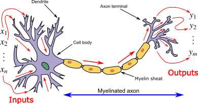
Neurons are organized into layers. There are generally three types of layers in a neural network:

• Input Layer: This layer receives the initial signals or input data. Each neuron in this layer represents a feature or input variable.
• Hidden Layers: These layers perform nonlinear transformations on the inputs. They are responsible for extracting and representing important features of the data. A neural network can have one or more hidden layers.
• Output Layer: This layer generates the network's output. The number of neurons in this layer depends on the nature of the task; for example, binary classification would have one output neuron, while multi-class classification would have several.

Training

The overall goal of training is to adjust the weights of the network so that it can generalize to new data, producing accurate results for examples it has not seen during training.

• Training data: Neural networks learn from examples. Each example consists of an "input" (the features) and a known "output" (the label or expected output).
• Error computation: When the network produces an output for a given input, the error is computed by comparing this output to the target output (the known result). There are different error measures, but the mean squared error (MSE) is commonly used.

Components of Artificial Neural Networks

• Neurons: Artificial neurons are the basic units of a neural network. Each neuron receives input signals, performs a computation on these signals using an activation function, and produces an output. Neurons are organized into layers: the input layer, hidden layers, and the output layer.
• Connections and Weights: The connections between neurons are represented by weights. Each connection has an associated weight that determines the relative importance of that connection in the computation of the output neuron. During training, these weights are adjusted to minimize the network's prediction error.
• Propagation Function (Forward Propagation): The propagation function, also called forward propagation, describes the process by which signals propagate through the network from the input layer to the output layer. Each neuron performs a transformation on the signals it receives, and these modified signals are transmitted to the neurons of the next layer.

Components of Artificial Neural Networks

Propagation Function

Activation Function: After computing the neuron's input, it is passed through an activation function. This function introduces nonlinearity into the model, allowing the neural network to capture complex relationships and learn nonlinear patterns. Some commonly used activation functions include:

• Sigmoid: \( \sigma(x) = \frac{1}{1 + e^{-x}} \)
• Hyperbolic tangent (tanh): \( \text{tanh}(x) = \frac{e^{x} - e^{-x}}{e^{x} + e^{-x}} \)
• ReLU (Rectified Linear Unit): \( \text{ReLU}(x) = \max(0, x) \)
• Softmax (for the output layer in classification): \( \text{Softmax}(x)_i = \frac{e^{x_i}}{\sum_{j} e^{x_j}} \)

Perceptron

The perceptron is a supervised learning algorithm used for binary classification. It is designed to solve problems where the objective is to determine whether a given input belongs to a particular class or not.

• The perceptron was invented by Frank Rosenblatt in 1958. The idea was to create a simple model of an artificial neuron inspired by the functioning of biological neurons. Rosenblatt formulated a learning algorithm that allows the perceptron to adjust its weights based on classification errors, thus improving its performance over time.

Perceptron: Formal Definition

• Let \(y = f(z)\) be the output of the perceptron for an input vector z
• Let \(N\) be the number of training examples
• Let X be the feature input space
• Let \({(x_{1}, d_{1}),...,(x_{N}, d_{N})}\) be the N training examples, where
  • \(x_i\) is the feature vector of the i^th training example.
  • \(d_i\) is the desired output value
  • \(x_{j,i}\) is the i^th feature of the j^th training example.
  • \(x_{j,0} = 1\)

Perceptron: Steps

1. Initialize the weights and thresholds
2. For each example, \((x_j, d_j)\) in the training set
   • Compute the current output: \[y_j(t)= f[w(t).x_j]\] \[= f[w_0(t)x_{j,0} + w_1(t)x_{j,1} + w_2(t)x_{j,2} + \dotsb + w_n(t)x_{j,n}]\]
   • Update the weight: \[w_i(t + 1) = w_i(t) + r. (d_j-y_j(t))x_{j,i}\]
   \(r\) is the learning rate.

Perceptron: Steps

3. Repeat step 2 until the iteration error \[\frac{1}{s} (Σ |d_j - y_j(t)|)\] is less than the user-specified threshold \(\gamma\), or a predetermined number of iterations have been performed, where \(s\) is again the size of the sample set.

• Stochastic Gradient Descent (SGD): update weights using gradient of loss on a mini-batch. \(w \leftarrow w - \eta \cdot \nabla L(w)\)
• Momentum SGD: accumulates velocity in gradient directions. \(v \leftarrow \beta v + \nabla L(w)\); \(w \leftarrow w - \eta \cdot v\)
• Adam optimizer: adaptive learning rates per parameter. Combines first moment (mean) and second moment (variance) of gradients. Default hyperparameters: \(\beta_1=0.9\), \(\beta_2=0.999\), \(\varepsilon=10^{-8}\).
• Learning rate: most critical hyperparameter. Too high → divergence; too low → slow convergence.
• Learning rate schedules: step decay, cosine annealing, warm-up.

• Weight initialization: Xavier/Glorot for sigmoid/tanh; He initialization for ReLU. Avoids vanishing/exploding gradients.
• Batch normalization: normalizes layer inputs to zero mean and unit variance. Improves training speed and stability.
• Layer normalization: normalizes across features (used in Transformers).
• Early stopping: halt training when validation loss stops improving. Prevents overfitting.
• Dropout: randomly zero a fraction p of neurons during training. Acts as regularization.
• Weight decay (L2 regularization): adds \(\lambda \cdot \|w\|^2\) penalty to the loss. Shrinks weights toward zero.

• Start with He initialization for ReLU networks
• Use Adam optimizer with default hyperparameters as a first attempt
• Add batch normalization after linear layers, before activation
• Monitor train and validation loss curves: if val loss diverges, apply dropout or weight decay
• Apply early stopping with a patience of 5–20 epochs
• Check gradient norms: if they explode, apply gradient clipping (max norm 1.0)
• For very deep networks, use residual connections (skip connections)

Multiclass perceptron

• The perceptron can be generalized to multiclass classification.
• A feature representation function \(f( x , y )\) maps each possible input/output pair to a finite-dimensional real-valued feature vector.
• The feature vector is multiplied by a weight vector \(w\), but the resulting score is now used to choose among many possible outcomes: \[\hat y = \operatorname{argmax}_y f(x,y) \cdot w.\]
• Re-learning is done by iterating over examples, predicting an outcome for each, leaving the weights unchanged when the predicted outcome matches the target, and modifying them when it does not. The update becomes: \[w_{t+1} = w_t + f(x, y) - f(x,\hat y)\].

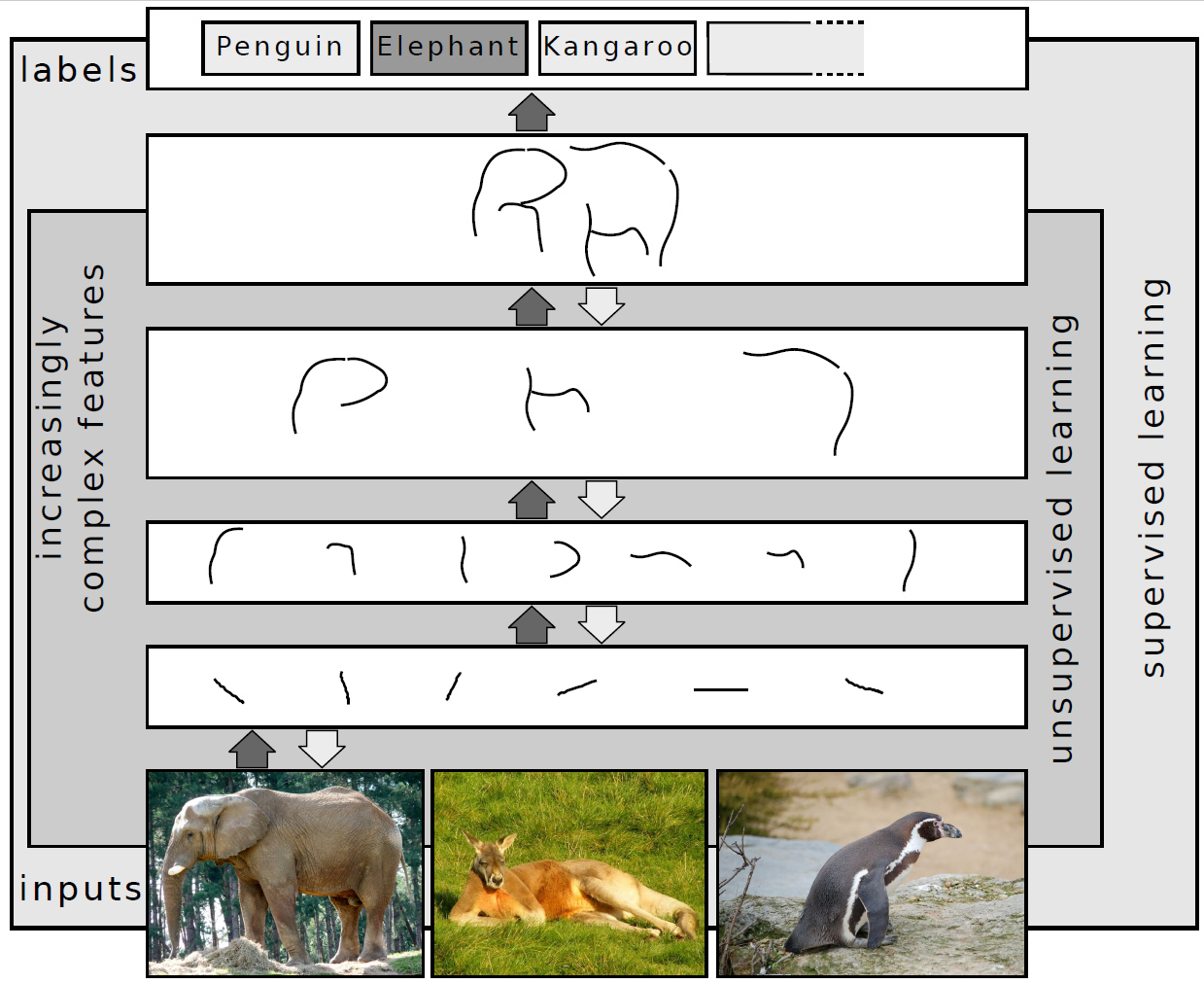
A deep neural network, also known as a deeply hierarchical neural network or deep neural network (DNN), is a type of artificial neural network that includes multiple processing layers, generally more than two. These networks are called "deep" because of their stacked layer architecture, enabling the creation of complex hierarchical representations of data.

Layered architecture: Deep neural networks are composed of multiple layers, generally divided into three main types:

• Input Layer: Receives the raw data or features as input.
• Hidden Layers: Perform nonlinear transformations and learn hierarchical representations of the data.
• Output Layer: Produces the network's output, adapted to the specific task (classification, regression, etc.).

• Hierarchical Learning: The hidden layers of a deep neural network learn increasingly abstract and complex features as depth increases. Each layer represents an abstraction of the features extracted by the previous layers.
• Activation Functions: Nonlinear activation functions, such as ReLU (Rectified Linear Unit) or its variants, are commonly used in hidden layers to allow the network to learn nonlinear relationships.
• Deep Learning: Deep learning involves the simultaneous adjustment of the weights of all layers in the network to minimize prediction error. This is typically achieved using backpropagation and gradient descent techniques.
• Applications: Deep neural networks are used in a variety of tasks, including computer vision, speech recognition, natural language processing, machine translation, content recommendation, and many others. Their ability to learn complex representations has led to significant advances in many areas of artificial intelligence.

Training deep neural networks may require large volumes of data and computing power.

Example: Tensorflow

# Step 3: Add a dense output layer with softmax activation function
# The layer has 2 neurons for a binary classification task, and softmax is used
# to obtain probabilities
model.add(Dense(units=2, activation='softmax'))

# Step 4: Compile the model
# Using stochastic gradient descent (SGD) as optimizer with a learning rate of 0.01
# The loss function is 'mean_squared_error' for a regression problem
# Model performance will be measured in terms of 'accuracy'
sgd = SGD(lr=0.01)
model.compile(loss='mean_squared_error', optimizer=sgd, metrics=['accuracy'])

Convolutional Neural Networks

Convolutional Neural Networks

Convolutional neural networks (CNNs) are a class of neural network architectures designed primarily for image analysis. They have been particularly effective in tasks such as image classification, object detection, and image segmentation.

• Image Analysis: CNNs are specifically designed to work with grid-structured data, such as images. They are capable of capturing important spatial patterns and features in images.

Convolutional Neural Networks

• Uses convolution: Convolution is a linear mathematical operation used to extract local features from an image. Convolution filters are applied to the image to detect patterns such as edges, textures, or shapes.
• Layered architecture: CNNs generally follow a layered architecture. They have an input layer to receive the image, one or more hidden layers composed mainly of convolutional layers, and an output layer to produce the final results.

Convolutional Neural Networks

• Convolutional layers: Convolutional layers are responsible for extracting features from the image. Each layer can have multiple convolution filters that learn to detect specific patterns. These layers are often followed by pooling layers to reduce the dimensionality of the representation while preserving important features.
• Applications: CNNs are widely used in applications such as image classification (e.g., recognizing animals in photos), object detection (locating and identifying specific objects), and image segmentation (dividing an image into semantically meaningful regions).

Convolutional Neural Networks: architecture

• Hierarchical data model: Convolutional neural networks (CNNs) are designed to capture hierarchical features in data, particularly in the context of image analysis. This means they can learn simple patterns in the early layers, then combine these patterns to form more complex features in subsequent layers.
• CNN architecture: A convolutional neural network is generally composed of an input layer, several hidden layers, and an output layer. The hidden layers consist mainly of convolutional layers, but can also include other types of layers such as pooling layers, fully connected layers, and normalization layers.

Convolutional Neural Networks: architecture

• Convolutional layers and activation function: Convolutional layers apply filters to extract features from the image. The multiplication is performed by the convolution. The most commonly used activation function is ReLU (Rectified Linear Unit), which introduces nonlinearity into the model. This nonlinearity is important to allow the network to learn complex relationships in the data.
• Additional layers: After the convolutional layers, one can have pooling layers to reduce dimensionality, fully connected layers to combine global features, and normalization layers to improve training stability.

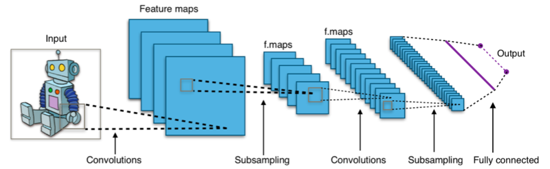
In summary, CNNs follow a hierarchical architecture, where convolutional layers learn local features, and these features are then combined in subsequent layers to form more complex representations. The nonlinearity introduced by the ReLU activation function is crucial to allow the model to learn nonlinear relationships in the data.

Kernel (image processing)

A kernel in the context of image processing, also called a filter or mask, is a small matrix that is applied to an image using a convolution operation. The purpose of applying these kernels is to perform various filtering operations on the image, such as edge detection, detail enhancement, highlighting certain features, etc.

• Convolution in CNNs: In CNNs, convolution is a key operation that consists of applying a set of filters (kernels) to an input image. Each filter is designed to extract specific features from the image, such as edges, textures, or other patterns.

Scientific datasets come in fundamentally different structural forms. The choice of architecture depends on the data modality.

Three main modalities in scientific contexts:

1. Time series / signals: measurements ordered in time or frequency (e.g., spectra, waveforms, sensor readings)
2. Images and spatial detectors: 2D or 3D grids (e.g., telescope images, microscopy, particle detector maps)
3. Tabular data: structured rows and features (e.g., catalog data, simulation parameters, measurement tables)

Note: This section is designated as asynchronous reading material.

• Sliding window approach: transform a 1D signal of length T into overlapping windows of size w → produces a 2D feature matrix of shape (N_windows, w).
• Feature extraction: mean, variance, FFT coefficients, spectral entropy, zero-crossing rate.
• 1D Convolutional Neural Network (1D-CNN): applies learned filters along the time axis. Efficient for local pattern detection in signals.
• Recurrent Neural Network (RNN) / LSTM: processes sequences step-by-step, maintaining hidden state. Suitable for long-range temporal dependencies.
• Example use case: classifying cosmic ray events from detector waveforms; detecting equipment faults from vibration signals.

Convolutional Neural Network (CNN): processes 2D grids using learned convolution filters. Key operations:

• Convolution: local feature detection (edges, textures, shapes)
• Pooling: spatial downsampling (max pool, average pool)
• Fully-connected layer: global classification/regression

• Transfer learning: pre-trained CNNs (ResNet, EfficientNet) can be fine-tuned on small scientific datasets.
• Example use case: galaxy morphology classification from telescope images; particle track reconstruction from detector readouts.
• When the spatial structure matters, CNNs are preferred over MLPs.

• Tabular data remains the most common format in scientific computing (simulations, catalogs, laboratory measurements).
• Classical ML (gradient boosting, random forests) often outperforms deep learning on tabular data, especially with < 10,000 samples.
• When to use deep learning for tabular data: very large datasets (>100k rows), complex feature interactions that cannot be manually engineered, multi-task learning.
• Embedding layers for categorical features: map discrete categories to continuous dense vectors.
• When NOT to use deep learning: small datasets, need for interpretability, structured data with well-understood features.

Reinforcement Learning

• Reinforcement Learning (RL) is a branch of machine learning inspired by theories of animal psychology.
• Autonomous agent: RL involves an autonomous agent interacting with an environment.
• Decision making: The agent makes decisions based on its current state.
• Rewards and penalties: The environment provides the agent with rewards, which can be positive or negative.
• Objective: The objective is to maximize the sum of cumulative rewards over time.

Licenses, Ethics and Privacy

• Data usage rights
• Confidentiality and privacy
• Ethics

• A well-calibrated model: if it predicts 70% probability for an event, that event should occur approximately 70% of the time.
• Calibration check: reliability diagram (calibration curve) — plot predicted probability vs. observed frequency. A perfectly calibrated model follows the diagonal.
• Common miscalibration: modern neural networks are often overconfident (predicted probabilities too extreme).
• Temperature scaling: divide logits by a scalar T > 0 before softmax. T > 1 softens predictions; T < 1 sharpens them. T is tuned on a validation set.
• Expected Calibration Error (ECE): measures average gap between confidence and accuracy across bins.

Types of uncertainty:

• Aleatoric uncertainty: inherent randomness in the data (irreducible). Cannot be reduced with more data.
• Epistemic uncertainty: model uncertainty due to limited training data (reducible with more data).

• Deep ensembles: train N independent models with different initializations. Aggregate predictions by averaging. Ensemble variance measures uncertainty.
• Bootstrap: resample training data N times, train N models. Confidence intervals from the distribution of predictions.
• Monte Carlo Dropout (MC Dropout): apply dropout at inference time with T forward passes. Mean = prediction; variance = uncertainty estimate. Low overhead, easily implemented.

Distribution shift: training and test data come from different distributions. Common in physics experiments (simulation ≠ real data).

Types:

• Covariate shift: P(x) changes, P(y|x) stays the same.
• Label shift: P(y) changes.
• Concept drift: P(y|x) changes over time.

Strategies:

• Domain adaptation: fine-tune on a small target-domain sample.
• Simulation-to-real (sim-to-real): train on simulation, validate with real data. Apply domain randomization to bridge the gap.
• Adversarial training: augment with perturbed samples to improve robustness.
• Stress tests / OOD detection: evaluate on shifted or corrupted inputs.

• Before training: check for systematic differences between train and test distributions (feature shift analysis, MMD test).
• During training: use data augmentation to simulate plausible distribution variations; apply domain randomization; mix simulation and real data where available.
• After training: run stress tests on corrupted or shifted inputs; monitor confidence scores — a drop in average confidence may signal distribution shift.
• OOD detection: models trained with softmax often assign high confidence to OOD inputs. Use energy-based scores or Mahalanobis distance for OOD detection.
• In experimental physics/astronomy: always validate on real data even when trained on Monte Carlo simulation; report calibration curves alongside accuracy.

Online Resources

• Artificial Neural Network
• Kernel (image processing)
• Convolutional neural network
• Perceptron

Colors

• Color Tool - Material Design

Images

• Wikimedia Commons