Data Science
John Samuel
CPE Lyon
Year: 2025-2026
Email: john.samuel@cpe.fr

John Samuel
CPE Lyon
Year: 2025-2026
Email: john.samuel@cpe.fr


.jpg)

This formalization is at the core of supervised learning, where the objective is to learn from labeled examples and find a function that can accurately predict labels for new unseen data.
Raw data rarely satisfies the assumptions of ML algorithms. Data preparation transforms the raw feature matrix into a form suitable for learning.
We use a small customer dataset for a marketing task: prepare the data before predicting high-value customers.
| customer_id | age | income | city | visits | annual_spend |
|---|---|---|---|---|---|
| C01 | 22 | 32000 | Paris | 4 | 420 |
| C02 | 25 | 36000 | Lyon | 5 | 510 |
| C03 | 29 | missing | Paris | 7 | 760 |
| C04 | 31 | 54000 | Marseille | 6 | 680 |
| C05 | 38 | 61000 | missing | 9 | 980 |
| C06 | 45 | 58000 | Lyon | 3 | 4800 |
Immediate issues: different scales, missing values, and an extreme spender (C06).
age, income, and annual_spend live on very different scales.
Without preprocessing, large-valued columns dominate.
city into binary columns.| customer_id | age | income | annual_spend | problem before preprocessing |
|---|---|---|---|---|
| C01 | 22 | 32000 | 420 | income dominates age |
| C03 | 29 | missing | 760 | missing income |
The following code prepares the numerical and categorical columns before model training.
prep = df.copy()
prep["income"] = prep["income"].fillna(prep["income"].median())
prep["city"] = prep["city"].fillna("Unknown")

scaled = prep[["age", "income", "annual_spend"]]
scaled = (scaled - scaled.mean()) / scaled.std(ddof=0)

city_dummies = pd.get_dummies(
    prep["city"], prefix="city", dtype=int
)
scaled contains standardized numerical columns, while city_dummies
contains binary variables for each city category.
After preprocessing, the numerical variables are comparable and the categorical variable becomes a set of binary columns.
| customer_id | age_z | income_z | spend_z | active city column |
|---|---|---|---|---|
| C01 | -1.24 | -1.55 | -0.61 | city_Paris = 1 |
| C04 | -0.09 | 0.44 | -0.44 | city_Marseille = 1 |
| C06 | 1.71 | 0.80 | 2.22 | city_Lyon = 1 |
Even after standardization, customer C06 still appears unusual because the spending
pattern is genuinely extreme, not just large in scale.
Here we keep a missing indicator, impute income with the median, and store missing cities as
Unknown.
| customer_id | income | income_missing | city | city_missing |
|---|---|---|---|---|
| C03 | 54000 | 1 | Paris | 0 |
| C05 | 61000 | 0 | Unknown | 1 |
Observed income median: 54000.
prep = df.copy()
prep["income_missing"] = prep["income"].isna().astype(int)
prep["city_missing"] = prep["city"].isna().astype(int)

prep["income"] = prep["income"].fillna(prep["income"].median())
prep["city"] = prep["city"].fillna("Unknown")

clean_subset = prep[[
    "customer_id", "income", "income_missing", "city", "city_missing"
]]
If the amount of missing data were tiny, we could also compare this approach with
df.dropna() and discuss the loss of observations.
The value 4800 is much larger than the other spending values. We cap it with the
IQR rule, then derive features that are easier for a model to exploit.
q1 = prep["annual_spend"].quantile(0.25)
q3 = prep["annual_spend"].quantile(0.75)
iqr = q3 - q1
upper = q3 + 1.5 * iqr

prep["annual_spend_capped"] = prep["annual_spend"].clip(upper=upper)
prep["spend_per_visit"] = (
    prep["annual_spend_capped"] / prep["visits"]
).round(1)
prep["is_high_value"] = (prep["annual_spend_capped"] >= 900).astype(int)
This creates one cleaned variable and two derived variables that are more directly useful for a classifier or a clustering algorithm.
| customer_id | annual_spend | capped | spend_per_visit | is_high_value |
|---|---|---|---|---|
| C05 | 980 | 980.00 | 108.9 | 1 |
| C06 | 4800 | 1483.75 | 494.6 | 1 |
Here, Q1 = 552.5, Q3 = 925.0, so the IQR upper bound is
1483.75. The new features summarize behavior more directly than the raw columns.

Suppose we classify emails into two categories using two features:
x = (contains_offer, exclamation_count).
| contains_offer | exclamation_count | true class | |
|---|---|---|---|
| E1 | 1 | 4 | spam |
| E2 | 1 | 1 | spam |
| E3 | 0 | 0 | not_spam |
| E4 | 0 | 1 | not_spam |
Choose one weight vector per class:
βspam = (2.0, 0.8) and
βnot_spam = (0.2, 0.1).
emails = pd.DataFrame({
    "email": ["E1", "E2", "E3", "E4"],
    "contains_offer": [1, 1, 0, 0],
    "exclamation_count": [4, 1, 0, 1],
})

beta_spam = [2.0, 0.8]
beta_not_spam = [0.2, 0.1]
X = emails[["contains_offer", "exclamation_count"]]

emails["score_spam"] = X.dot(beta_spam)
emails["score_not_spam"] = X.dot(beta_not_spam)
emails["predicted_class"] = np.where(
    emails["score_spam"] > emails["score_not_spam"], "spam", "not_spam"
)
This produces one score per class for every email.
| score_spam | score_not_spam | predicted class | |
|---|---|---|---|
| E1 | 5.2 | 0.6 | spam |
| E2 | 2.8 | 0.3 | spam |
| E3 | 0.0 | 0.0 | not_spam |
| E4 | 0.8 | 0.1 | spam |
The class with the highest dot-product score is selected for each email; ties are sent to
not_spam here.
Reflection: E4 is predicted as spam even though its true class is
not_spam. This is useful: a linear classifier is simple and interpretable, but with
only two features it may confuse legitimate but emphatic emails with spam.


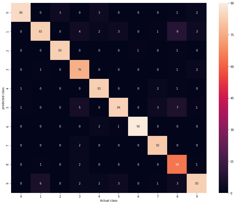
The confusion matrix is an essential tool for evaluating the performance of a classification system. It provides a detailed view of the predictions made by the model relative to the actual classes.
We predict whether a student passes using hours_studied and exercise_score.
from sklearn.linear_model import LogisticRegression
from sklearn.metrics import confusion_matrix

binary = pd.DataFrame({...})
Xb = binary[["hours_studied", "exercise_score"]]
yb = binary["passed"]model_b = LogisticRegression(random_state=0).fit(Xb, yb)
pred_b = model_b.predict(Xb)
cm_b = confusion_matrix(yb, pred_b)The result is [[3, 1], [1, 3]]: one false positive and one false negative.
| Predicted 0 | Predicted 1 | |
|---|---|---|
| Actual 0 | 3 | 1 |
| Actual 1 | 1 | 3 |
The same idea extends to three classes. Here we classify students into
Arts, Literature, and Science.
multi = pd.DataFrame({
    "math_score": [2, 3, 4, 6, 7, 8, 4, 5, 6],
    "writing_score": [8, 7, 6, 5, 4, 3, 5, 6, 4],
    "track": ["Literature", "Literature", "Literature", "Science", "Science", "Science", "Arts", "Arts", "Arts"],
})

Xm = multi[["math_score", "writing_score"]]
ym = multi["track"]
model_m = LogisticRegression(random_state=0, max_iter=1000).fit(Xm, ym)
pred_m = model_m.predict(Xm)
cm_m = confusion_matrix(ym, pred_m, labels=["Arts", "Literature", "Science"])
The matrix is
[[2, 0, 1], [0, 3, 0], [0, 0, 3]]: most predictions are correct, but one
Arts student is confused with Science.

The Support Vector Machine (SVM) is a supervised learning method. SVM seeks to find the best decision boundary that optimizes class separation, allowing accurate classification even in complex data spaces.

The hyperplane in n-dimensional space is an (n-1)-dimensional subspace that separates the data into two classes.

| point | x1 | x2 | class |
|---|---|---|---|
| P1 | 1 | 7 | -1 |
| P2 | 2 | 6 | -1 |
| P3 | 2 | 5 | -1 |
| P4 | 3 | 6 | -1 |
| P5 | 4 | 3 | +1 |
| P6 | 5 | 2 | +1 |
| P7 | 5 | 3 | +1 |
| P8 | 6 | 2 | +1 |
-1 and +1 can be split by
one
straight line.from sklearn.svm import SVC
svm_df = pd.DataFrame({
"x1": [1, 2, 2, 3, 4, 5, 5, 6],
"x2": [7, 6, 5, 6, 3, 2, 3, 2],
"label": [-1, -1, -1, -1, 1, 1, 1, 1],
})
X = svm_df[["x1", "x2"]]
y = svm_df["label"]
svm_model = SVC(kernel="linear", C=1.0).fit(X, y)
w = svm_model.coef_[0]
b = -svm_model.intercept_[0]
support = svm_model.support_vectors_x2 = x1 + 1, with support vectors
near
(2, 5) and (4, 3).
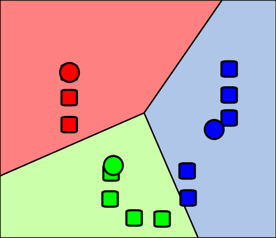
The k-nearest neighbors (kNN) method and k-means clustering are two important techniques in machine learning and data mining:
The k-nearest neighbors (k-NN) method is a supervised learning algorithm used for both classification and regression.
| customer | age | visits | segment | spend_per_visit |
|---|---|---|---|---|
| C1 | 23 | 2 | Occasional | 35 |
| C2 | 25 | 3 | Occasional | 40 |
| C3 | 28 | 4 | Regular | 55 |
| C4 | 35 | 7 | Regular | 75 |
| C5 | 38 | 8 | Premium | 95 |
| C6 | 42 | 9 | Premium | 110 |
We study a new customer with (age=30, visits=6) using k = 3.
The algorithm will compare this point with the stored customers and use the three closest neighbors to make a prediction.
from sklearn.neighbors import KNeighborsClassifier

customers = pd.DataFrame({...})
X = customers[["age", "visits"]]
y_class = customers["segment"]

knn_clf = KNeighborsClassifier(n_neighbors=3)
knn_clf.fit(X, y_class)

new_customer = pd.DataFrame({"age": [30], "visits": [6]})
predicted_segment = knn_clf.predict(new_customer)[0]C3, C4, and C2.Regular, Regular, Occasional.
Regular.from sklearn.neighbors import KNeighborsRegressor
y_reg = customers["spend_per_visit"]
knn_reg = KNeighborsRegressor(n_neighbors=3)
knn_reg.fit(X, y_reg)
predicted_spend = knn_reg.predict(new_customer)[0]The same neighbors (C3, C4, C2) have spend values
55, 75, and 40.
The regression prediction is their average:
(55 + 75 + 40) / 3 = 56.7.
This is the key difference: classification votes on labels, while regression averages numerical targets.
Consider labeled 2D training points. We want to classify the new point \((4, 3)\).
points = pd.DataFrame({...})
new_point = pd.DataFrame({"x": [4], "y": [3]})| Point | x coordinate | y coordinate | Class |
|---|---|---|---|
| A | 2 | 3 | Red |
| B | 4 | 4 | Red |
| C | 3 | 2 | Blue |
| D | 6 | 5 | Red |
| E | 5 | 3 | Blue |
from sklearn.neighbors import KNeighborsClassifier

points["distance"] = ((points["x"] - 4)**2 + (points["y"] - 3)**2)**0.5
knn = KNeighborsClassifier(n_neighbors=3)
knn.fit(points[["x", "y"]], points["label"])
prediction = knn.predict(new_point)[0]k = 3.B, E, and C.Blue.Naive Bayes classification is a simple probabilistic classification method based on the application of Bayes' theorem with a strong independence assumption between features.
\[ P(C \mid x)=\frac{P(x \mid C)P(C)}{P(x)} \]
P(C) is the prior, P(x | C) the likelihood,
and
P(C | x) the posterior.
C, the features are treated as independent.\[ P(x_1,\dots,x_d \mid C)\approx \prod_{i=1}^{d} P(x_i \mid C) \]
Prediction rule: \(\hat{C}=\arg\max_C P(C)\prod_i P(x_i \mid C)\).
We encode short email messages as binary features and train a Bernoulli Naive Bayes classifier.
| contains_free | contains_win | many_caps | label | |
|---|---|---|---|---|
| E1 | 1 | 1 | 1 | spam |
| E2 | 1 | 0 | 1 | spam |
| E3 | 0 | 0 | 0 | ham |
| E4 | 0 | 0 | 1 | ham |
| E5 | 1 | 1 | 0 | spam |
The independence assumption means the model combines the evidence from each feature as if they were conditionally independent given the class.
emails = pd.DataFrame({
    "contains_free": [1, 1, 0, 0, 1],
    "contains_win": [1, 0, 0, 0, 1],
    "many_caps": [1, 1, 0, 1, 0],
    "label": ["spam", "spam", "ham", "ham", "spam"],
})

X = emails[["contains_free", "contains_win", "many_caps"]]
y = emails["label"]
model = BernoulliNB()
model.fit(X, y)new_messages = pd.DataFrame({
"contains_free": [1, 0],
"contains_win": [0, 1],
"many_caps": [1, 0],
}, index=["M1", "M2"])
pred = model.predict(new_messages)
proba = model.predict_proba(new_messages)| message | features | predicted class | comment |
|---|---|---|---|
| M1 | (1, 0, 1) | spam | free and capitals push the posterior toward spam |
| M2 | (0, 1, 0) | spam | win is rare in ham and increases spam probability |
Naive Bayes estimates \(P(class \mid features)\) and chooses the largest posterior. Even with a tiny dataset, we can explain the prediction by looking at how each observed feature changes the class probability.
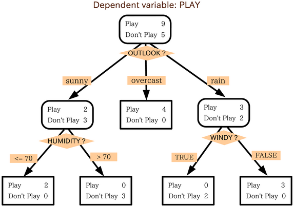
Decision trees represent decisions and consequences as a tree.
| applicant | income_k | debt_ratio | late_payments | approved |
|---|---|---|---|---|
| A1 | 32 | 0.52 | 4 | no |
| A2 | 58 | 0.18 | 0 | yes |
| A3 | 45 | 0.30 | 1 | yes |
| A4 | 28 | 0.61 | 3 | no |
| A5 | 64 | 0.25 | 0 | yes |
The tree tests candidate splits such as debt_ratio < 0.4 or
late_payments < 2 and keeps the split that best separates yes from
no.
loan = pd.DataFrame({
    "income_k": [32, 58, 45, 28, 64],
    "debt_ratio": [0.52, 0.18, 0.30, 0.61, 0.25],
    "late_payments": [4, 0, 1, 3, 0],
    "approved": ["no", "yes", "yes", "no", "yes"],
})

X = loan[["income_k", "debt_ratio", "late_payments"]]
y = loan["approved"]
tree = DecisionTreeClassifier(criterion="gini", max_depth=2, random_state=0)
tree.fit(X, y)
At each node, the classifier checks several thresholds and keeps the split with the largest impurity reduction.
rules = export_text(tree, feature_names=list(X.columns))

# possible simplified output
|--- debt_ratio <= 0.41
|   |--- late_payments <= 1.50: yes
|   |--- late_payments > 1.50: no
|--- debt_ratio > 0.41: no
The root split is most informative; later splits refine only the remaining mixed groups.
Example of building: at the root, a split like debt_ratio ≤ 0.41
is useful because it puts A2,A3,A5 on one side and all three are yes,
while A1,A4 go to the other side and both are no. The child nodes are then
split again only if they still contain mixed labels.
In the context of decision trees, data is generally represented as vectors where each element of the vector corresponds to a feature or independent variable, and the dependent variable is the target that one seeks to predict or classify.
Ensemble learning, in particular random forests, is a technique that combines multiple learning models to improve predictive performance compared to a single model. Random forests are obtained by building multiple decision trees during the training phase.
Suppose we predict whether a customer will default using spending and repayment behaviour.
| customer | income_k | balance_k | missed_payments | default |
|---|---|---|---|---|
| C1 | 70 | 5 | 0 | no |
| C2 | 42 | 16 | 2 | yes |
| C3 | 90 | 7 | 0 | no |
| C4 | 38 | 18 | 3 | yes |
| C5 | 55 | 10 | 1 | no |
Each tree sees a slightly different bootstrap sample, so the final model relies on many weakly different decision rules instead of 1 fragile tree.
credit = pd.DataFrame({
    "income_k": [70, 42, 90, 38, 55, 48, 80, 36],
    "balance_k": [5, 16, 7, 18, 10, 14, 6, 20],
    "missed_payments": [0, 2, 0, 3, 1, 2, 0, 4],
    "default": ["no", "yes", "no", "yes", "no", "yes", "no", "yes"],
})

X = credit[["income_k", "balance_k", "missed_payments"]]
y = credit["default"]
This slide prepares the training data: X contains the input
features, and y contains the label to predict, namely whether the customer defaults.
forest = RandomForestClassifier(n_estimators=50, max_depth=3, random_state=0)
forest.fit(X, y)

importance = pd.Series(forest.feature_importances_, index=X.columns).sort_values(ascending=False)
After fitting many trees, the forest estimates which features were most useful
for separating default=yes from default=no.
For a new customer with income_k=50, balance_k=15,
missed_payments=2:
yes for default risk in this example.
missed_payments and
balance_k above income_k, which matches domain intuition.
This is the practical value of ensemble learning: lower variance and more robust predictions.

Linear regression is a mathematical model that represents a linear relationship between an independent variable \(x_i\) and a dependent variable \(y_i\). The model takes the form of a straight line (for simple linear regression) or a parabola (for multiple linear regression).
Straight line: \(y_i = β_0 + β_1x_i + ε_i\) where \(β_0\) and \(β_1\) are the regression coefficients, \(x_i\) is the independent variable, and \(ε_i\) is the residual error.
To minimize the error:
The objective is to minimize SSE to obtain the best approximation of the linear relationship between variables.
SGD is an iterative method that updates the model to reduce a loss function, often one example at a time.
For regression, the objective is often the average loss over the dataset: \[ J(w)=\frac{1}{n}\sum_{i=1}^{n} L(w;x_i,y_i) \]
\(J(w)\) is the total objective, and \(L(w;x_i,y_i)\) is the error on one training example.
| flat | surface_m2 | distance_km | rooms | rent_eur |
|---|---|---|---|---|
| F1 | 28 | 7.5 | 1 | 820 |
| F2 | 35 | 5.0 | 2 | 980 |
| F3 | 52 | 3.0 | 2 | 1350 |
| F4 | 65 | 2.0 | 3 | 1680 |
| F5 | 42 | 6.5 | 2 | 1100 |
We model rent with a linear prediction such as \(\hat{y}=w_1x_1+w_2x_2+w_3x_3+b\), where the features are surface, distance, and rooms.
A common loss for one apartment is the squared error \(L(w;x_i,y_i)=(\hat{y}_i-y_i)^2\), so large mistakes receive a larger penalty.
rent = pd.DataFrame({
    "surface_m2": [28, 35, 52, 65, 42, 58, 31, 47],
    "distance_km": [7.5, 5.0, 3.0, 2.0, 6.5, 4.0, 8.0, 3.5],
    "rooms": [1, 2, 2, 3, 2, 3, 1, 2],
    "rent_eur": [820, 980, 1350, 1680, 1100, 1490, 860, 1280],
})

X = rent[["surface_m2", "distance_km", "rooms"]]
y = rent["rent_eur"]
scaler = StandardScaler()
X_scaled = scaler.fit_transform(X)
Now SGD uses one training example at a time to reduce the loss: \(w \leftarrow w - \eta \nabla L(w;x_i,y_i)\).
Here, \(\nabla L\) tells us which direction increases error, and \(\eta\) controls how large the correction step is. Scaling keeps one feature from dominating the update.
sgd = SGDRegressor(max_iter=20000, eta0=0.01, learning_rate="adaptive", random_state=0)
sgd.fit(X_scaled, y)surface_m2=50, distance_km=4, and
rooms=2, we transform the features with the same scaler and call
sgd.predict(...).
surface_m2 means larger flats increase rent, while a
negative coefficient for distance_km means locations farther from the center tend
to reduce rent.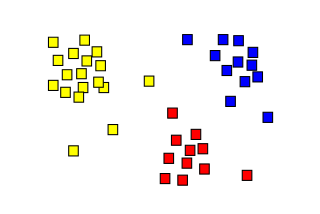
\[ C_1.. ∪ ..C_k ∪ C_{outliers} = X \] and
\[ C_i ∩ C_j = ϕ, i ≠ j; 1 <i,j <k \]
\(C_{outliers}\) may consist of extreme cases (data anomalies)
| customer | annual_spend | visits_per_month |
|---|---|---|
| C1 | 220 | 2 |
| C2 | 260 | 3 |
| C3 | 980 | 12 |
| C4 | 1020 | 11 |
| C5 | 540 | 6 |
| C6 | 560 | 7 |
The data are unlabeled. We want the algorithm to discover groups such as low-, medium-, and high-value customers.
segments = pd.DataFrame({
    "annual_spend": [220, 260, 980, 1020, 540, 560, 2400],
    "visits_per_month": [2, 3, 12, 11, 6, 7, 1],
}, index=["C1", "C2", "C3", "C4", "C5", "C6", "C7"])

kmeans = KMeans(n_clusters=3, random_state=0, n_init=10)
segments["kmeans_cluster"] = kmeans.fit_predict(segments)3 clusters before learning begins.dbscan = DBSCAN(eps=180, min_samples=2)
segments["dbscan_cluster"] = dbscan.fit_predict(segments[["annual_spend", "visits_per_month"]])
sil = silhouette_score(segments[["annual_spend", "visits_per_month"]], segments["kmeans_cluster"])eps.-1.C7 is far from the dense customer groups, so DBSCAN can treat it
as noise.-1 means "noise" rather than "force into a
cluster".Anomaly detection, also known as outlier detection, involves identifying unusual or divergent data in a dataset. Here are some common approaches to detecting anomalies:
Unexpected spikes: Anomalies can manifest as unexpected spikes or bursts in data. For example, a sudden increase in web traffic may indicate a denial of service (DDoS) attack in the case of network traffic monitoring, or an abnormal increase in financial transactions may signal fraud.
The characteristics of data vary depending on the application domain and the specific types of anomalies sought. Identifying unusual patterns or aberrant behaviors in data can help detect anomalies and take appropriate measures to manage them.
Anomaly detection algorithms identify rare observations that differ significantly from the majority of the data.
transactions = pd.DataFrame({
    "amount_eur": [18, 22, 25, 31, 410, 27, 19, 520],
    "login_gap_min": [120, 95, 80, 110, 2, 105, 130, 1],
}, index=["T1", "T2", "T3", "T4", "T5", "T6", "T7", "T8"])

features = transactions.copy()

iso = IsolationForest(contamination=0.25, random_state=0)
transactions["anomaly_flag"] = iso.fit_predict(features)
transactions["anomaly_score"] = iso.decision_function(features)
transactions.sort_values("anomaly_score")
fit_predict builds many random trees and labels likely anomalies as
-1.T5 and
T8 easier to isolate than typical transactions.| transaction | flag | interpretation |
|---|---|---|
| T5 | -1 | large amount and very short delay after login |
| T8 | -1 | another isolated point with extreme behaviour |
| T1-T4, T6-T7 | 1 | closer to normal transaction patterns |
Isolation Forest builds many random trees. Unusual points get isolated after only a few splits, so they have shorter average path lengths and lower scores.
Feature selection is a process aimed at choosing a subset of relevant features from a large number of available features.
customers = pd.DataFrame({
    "visits": [2, 3, 9, 10, 4, 8, 1, 7],
    "avg_basket": [18, 22, 65, 72, 25, 60, 15, 58],
    "support_calls": [5, 4, 1, 0, 3, 1, 6, 1],
    "coupon_clicks": [0, 1, 6, 5, 1, 4, 0, 5],
    "loyal": [0, 0, 1, 1, 0, 1, 0, 1],
})

X = customers.drop(columns="loyal")
y = customers["loyal"]
selector = SelectKBest(score_func=f_classif, k=2)
X_selected = selector.fit_transform(X, y)
selected_features = X.columns[selector.get_support()]
The idea is to keep only the variables that best separate loyal and non-loyal customers.
selected_features = ["avg_basket", "coupon_clicks"], these are the two
strongest variables under the chosen scoring rule.A typical ML project moves from question to monitored model.
Translating a scientific question into a well-defined ML problem is a critical first step. The choice of problem type determines which algorithms, metrics, and evaluation strategies are appropriate.
Proper data partitioning is essential to obtain unbiased estimates of model performance and to avoid overfitting.
Cross-validation is a resampling technique used to evaluate a model's generalization performance when the dataset is too small for a separate validation set.
This section introduced advanced topics in the data science and machine learning workflow.