Working with Tensorflow and Tensorflow datasets

import tensorflow as tf

import tensorflow_datasets as tfds

List all the available datasets

tfds.list_builders()

['abstract_reasoning',
 'accentdb',
 'aeslc',
 'aflw2k3d',
 'ag_news_subset',
 'ai2_arc',
 'ai2_arc_with_ir',
 'amazon_us_reviews',
 'anli',
 'arc',
 'bair_robot_pushing_small',
 'bccd',
 'beans',
 'big_patent',
 'bigearthnet',
 'billsum',
 'binarized_mnist',
 'binary_alpha_digits',
 'blimp',
 'bool_q',
 'c4',
 'caltech101',
 'caltech_birds2010',
 'caltech_birds2011',
 'cars196',
 'cassava',
 'cats_vs_dogs',
 'celeb_a',
 'celeb_a_hq',
 'cfq',
 'chexpert',
 'cifar10',
 'cifar100',
 'cifar10_1',
 'cifar10_corrupted',
 'citrus_leaves',
 'cityscapes',
 'civil_comments',
 'clevr',
 'clic',
 'clinc_oos',
 'cmaterdb',
 'cnn_dailymail',
 'coco',
 'coco_captions',
 'coil100',
 'colorectal_histology',
 'colorectal_histology_large',
 'common_voice',
 'coqa',
 'cos_e',
 'cosmos_qa',
 'covid19sum',
 'crema_d',
 'curated_breast_imaging_ddsm',
 'cycle_gan',
 'deep_weeds',
 'definite_pronoun_resolution',
 'dementiabank',
 'diabetic_retinopathy_detection',
 'div2k',
 'dmlab',
 'downsampled_imagenet',
 'dsprites',
 'dtd',
 'duke_ultrasound',
 'emnist',
 'eraser_multi_rc',
 'esnli',
 'eurosat',
 'fashion_mnist',
 'flic',
 'flores',
 'food101',
 'forest_fires',
 'fuss',
 'gap',
 'geirhos_conflict_stimuli',
 'genomics_ood',
 'german_credit_numeric',
 'gigaword',
 'glue',
 'goemotions',
 'gpt3',
 'groove',
 'gtzan',
 'gtzan_music_speech',
 'hellaswag',
 'higgs',
 'horses_or_humans',
 'i_naturalist2017',
 'imagenet2012',
 'imagenet2012_corrupted',
 'imagenet2012_real',
 'imagenet2012_subset',
 'imagenet_a',
 'imagenet_r',
 'imagenet_resized',
 'imagenet_v2',
 'imagenette',
 'imagewang',
 'imdb_reviews',
 'irc_disentanglement',
 'iris',
 'kitti',
 'kmnist',
 'lfw',
 'librispeech',
 'librispeech_lm',
 'libritts',
 'ljspeech',
 'lm1b',
 'lost_and_found',
 'lsun',
 'malaria',
 'math_dataset',
 'mctaco',
 'mnist',
 'mnist_corrupted',
 'movie_lens',
 'movie_rationales',
 'movielens',
 'moving_mnist',
 'multi_news',
 'multi_nli',
 'multi_nli_mismatch',
 'natural_questions',
 'natural_questions_open',
 'newsroom',
 'nsynth',
 'nyu_depth_v2',
 'omniglot',
 'open_images_challenge2019_detection',
 'open_images_v4',
 'openbookqa',
 'opinion_abstracts',
 'opinosis',
 'opus',
 'oxford_flowers102',
 'oxford_iiit_pet',
 'para_crawl',
 'patch_camelyon',
 'paws_wiki',
 'paws_x_wiki',
 'pet_finder',
 'pg19',
 'places365_small',
 'plant_leaves',
 'plant_village',
 'plantae_k',
 'qa4mre',
 'qasc',
 'quickdraw_bitmap',
 'radon',
 'reddit',
 'reddit_disentanglement',
 'reddit_tifu',
 'resisc45',
 'robonet',
 'rock_paper_scissors',
 'rock_you',
 'salient_span_wikipedia',
 'samsum',
 'savee',
 'scan',
 'scene_parse150',
 'scicite',
 'scientific_papers',
 'sentiment140',
 'shapes3d',
 'smallnorb',
 'snli',
 'so2sat',
 'speech_commands',
 'spoken_digit',
 'squad',
 'stanford_dogs',
 'stanford_online_products',
 'starcraft_video',
 'stl10',
 'sun397',
 'super_glue',
 'svhn_cropped',
 'ted_hrlr_translate',
 'ted_multi_translate',
 'tedlium',
 'tf_flowers',
 'the300w_lp',
 'tiny_shakespeare',
 'titanic',
 'trec',
 'trivia_qa',
 'tydi_qa',
 'uc_merced',
 'ucf101',
 'vctk',
 'vgg_face2',
 'visual_domain_decathlon',
 'voc',
 'voxceleb',
 'voxforge',
 'waymo_open_dataset',
 'web_questions',
 'wider_face',
 'wiki40b',
 'wikihow',
 'wikipedia',
 'wikipedia_toxicity_subtypes',
 'wine_quality',
 'winogrande',
 'wmt14_translate',
 'wmt15_translate',
 'wmt16_translate',
 'wmt17_translate',
 'wmt18_translate',
 'wmt19_translate',
 'wmt_t2t_translate',
 'wmt_translate',
 'wordnet',
 'xnli',
 'xquad',
 'xsum',
 'yelp_polarity_reviews',
 'yes_no']

Dataset Information

We will first use tfds.builder to obtain information related to a dataset like MNIST. Take a look at the available information for this dataset, especially the available features (features) and the total number of examples (total_num_examples).

builder = tfds.builder("mnist")
print(builder.info)

tfds.core.DatasetInfo(
    name='mnist',
    version=3.0.1,
    description='The MNIST database of handwritten digits.',
    homepage='http://yann.lecun.com/exdb/mnist/',
    features=FeaturesDict({
        'image': Image(shape=(28, 28, 1), dtype=tf.uint8),
        'label': ClassLabel(shape=(), dtype=tf.int64, num_classes=10),
    }),
    total_num_examples=70000,
    splits={
        'test': 10000,
        'train': 60000,
    },
    supervised_keys=('image', 'label'),
    citation="""@article{lecun2010mnist,
      title={MNIST handwritten digit database},
      author={LeCun, Yann and Cortes, Corinna and Burges, CJ},
      journal={ATT Labs [Online]. Available: http://yann.lecun.com/exdb/mnist},
      volume={2},
      year={2010}
    }""",
    redistribution_info=,
)

Features

builder = tfds.builder("mnist")
print(builder.info.features)

FeaturesDict({
    'image': Image(shape=(28, 28, 1), dtype=tf.uint8),
    'label': ClassLabel(shape=(), dtype=tf.int64, num_classes=10),
})

Label details

builder = tfds.builder("mnist")

# Number of classes
print(builder.info.features["label"].num_classes)

# Class names
print(builder.info.features["label"].names)

# Get the number equiavalent to a label
print(builder.info.features["label"].str2int("8"))

# shape
print(builder.info.features.shape)

# type of label
print(builder.info.features["label"].dtype)

10
['0', '1', '2', '3', '4', '5', '6', '7', '8', '9']
8
{'image': (28, 28, 1), 'label': ()}
<dtype: 'int64'>

Features of different datasets

Remove the break from the following code and see the available features from the different datasets.

for dataset in tfds.list_builders():
    builder = tfds.builder(dataset)
    print(
        f"Name: {{0}}\n description: {{1}}".format(
            builder.info.name, builder.info.description
        )
    )
    print(f"Name: {{0}}".format(builder.info.features))
    break

Name: abstract_reasoning
 description: Procedurally Generated Matrices (PGM) data from the paper Measuring Abstract Reasoning in Neural Networks, Barrett, Hill, Santoro et al. 2018. The goal is to infer the correct answer from the context panels based on abstract reasoning.

To use this data set, please download all the *.tar.gz files from the data set page and place them in ~/tensorflow_datasets/abstract_reasoning/.

$R$ denotes the set of relation types (progression, XOR, OR, AND, consistent union), $O$ denotes the object types (shape, line), and $A$ denotes the attribute types (size, colour, position, number). The structure of a matrix, $S$, is the set of triples $S={[r, o, a]}$ that determine the challenge posed by a particular matrix.
Name: FeaturesDict({
    'answers': Video(Image(shape=(160, 160, 1), dtype=tf.uint8)),
    'context': Video(Image(shape=(160, 160, 1), dtype=tf.uint8)),
    'filename': Text(shape=(), dtype=tf.string),
    'meta_target': Tensor(shape=(12,), dtype=tf.int64),
    'relation_structure_encoded': Tensor(shape=(4, 12), dtype=tf.int64),
    'target': ClassLabel(shape=(), dtype=tf.int64, num_classes=8),
})

Loading a dataset

Let’s start with loading the MNIST dataset for handwriting recognition

ds = tfds.load("mnist", split="train", shuffle_files=True, try_gcs=True)
assert isinstance(ds, tf.data.Dataset)
print(ds)

<_OptionsDataset shapes: {image: (28, 28, 1), label: ()}, types: {image: tf.uint8, label: tf.int64}>

Iterate over a dataset. Each entry in the dataset has 2 parts: image of a handwritten digit and the associated label.

for example in ds:  # example is `{'image': tf.Tensor, 'label': tf.Tensor}`
    print(list(example.keys()))
    image = example["image"]
    label = example["label"]
    print(image.shape, label)
    break

['image', 'label']
(28, 28, 1) tf.Tensor(1, shape=(), dtype=int64)

Obtain a tuple

ds = tfds.load("mnist", split="train", as_supervised=True, try_gcs=True)

for image, label in ds:  # example is (image, label)
    print(label)
    break

tf.Tensor(4, shape=(), dtype=int64)

Visualization

Another way is to use take() and pass a number n to select n examples from the dataset. Passing with_info with True helps to create the dataframe with necessary information for the visualization. Try changing the value of with_info to False and see the errors.

ds, info = tfds.load("mnist", split="train", with_info=True, try_gcs=True)

tfds.as_dataframe(ds.take(1), info)

	image	label
0		4

Change the parameter value of ds.take().

ds, info = tfds.load("mnist", split="train", with_info=True, try_gcs=True)

tfds.as_dataframe(ds.take(10), info)

	image	label
0		4
1		1
2		0
3		7
4		8
5		1
6		2
7		7
8		1
9		6

Splitting datasets for training and testing

For tasks like classification, it is important to classify the data for training and testing. There are several ways it can be done. In the following example, we display the information of the dataset after the loading of the dataset. Take a look at different information like features, splits, total_num_examples etc.

(ds_train, ds_test), info = tfds.load("mnist", split=["train", "test"], with_info=True)
print(info)

tfds.core.DatasetInfo(
    name='mnist',
    version=3.0.1,
    description='The MNIST database of handwritten digits.',
    homepage='http://yann.lecun.com/exdb/mnist/',
    features=FeaturesDict({
        'image': Image(shape=(28, 28, 1), dtype=tf.uint8),
        'label': ClassLabel(shape=(), dtype=tf.int64, num_classes=10),
    }),
    total_num_examples=70000,
    splits={
        'test': 10000,
        'train': 60000,
    },
    supervised_keys=('image', 'label'),
    citation="""@article{lecun2010mnist,
      title={MNIST handwritten digit database},
      author={LeCun, Yann and Cortes, Corinna and Burges, CJ},
      journal={ATT Labs [Online]. Available: http://yann.lecun.com/exdb/mnist},
      volume={2},
      year={2010}
    }""",
    redistribution_info=,
)

To create a training dataset from the first 80% of the training split.

ds_train, info = tfds.load("mnist", split="train[80%:]", with_info=True)

Applying modifications

def normalize_img(image, label):
    """Normalizes images: `uint8` -> `float32`."""
    return tf.cast(image, tf.float32) / 255.0, label


(ds_train, ds_test), info = tfds.load(
    "mnist", split=["train", "test"], as_supervised=True, with_info=True
)
ds_train = ds_train.map(normalize_img)
ds_test = ds_test.map(normalize_img)

Batches

For testing and training, it is important to create batches. Make use of batch() for creating batches of the specified size. For example, the code below will create batches of 128 samples.

(ds_train, ds_test), info = tfds.load(
    "mnist", split=["train", "test"], as_supervised=True, with_info=True
)
ds_train = ds_train.batch(128)
ds_test = ds_test.batch(128)
print(ds_train)
print(ds_test)

<BatchDataset shapes: ((None, 28, 28, 1), (None,)), types: (tf.uint8, tf.int64)>
<BatchDataset shapes: ((None, 28, 28, 1), (None,)), types: (tf.uint8, tf.int64)>

Building a training model

model = tf.keras.models.Sequential(
    [
        tf.keras.layers.Flatten(input_shape=info.features["image"].shape),
        tf.keras.layers.Dense(128, activation="relu"),
        tf.keras.layers.Dense(10, activation="softmax"),
    ]
)

model.compile(
    loss="sparse_categorical_crossentropy",
    optimizer=tf.keras.optimizers.Adam(0.001),
    metrics=["accuracy"],
)

Model Summary

print(model.summary())

Model: "sequential"
_________________________________________________________________
Layer (type)                 Output Shape              Param #   
=================================================================
flatten (Flatten)            (None, 784)               0         
_________________________________________________________________
dense (Dense)                (None, 128)               100480    
_________________________________________________________________
dense_1 (Dense)              (None, 10)                1290      
=================================================================
Total params: 101,770
Trainable params: 101,770
Non-trainable params: 0
_________________________________________________________________
None

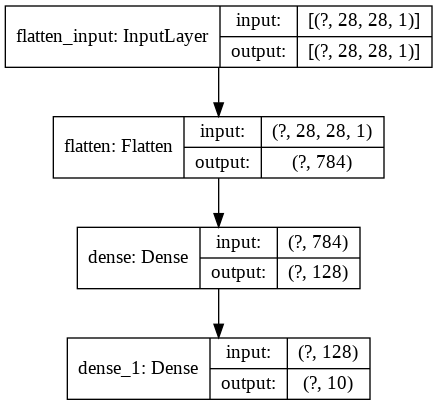
Visualizing the model

from tensorflow.keras.utils import plot_model

plot_model(model, show_shapes=True)

Training

history = model.fit(ds_train, epochs=10, batch_size=10, validation_data=ds_test)

Epoch 1/10
469/469 [==============================] - 9s 18ms/step - loss: 4.5828 - accuracy: 0.8607 - val_loss: 1.0424 - val_accuracy: 0.8870
Epoch 2/10
469/469 [==============================] - 2s 4ms/step - loss: 0.6286 - accuracy: 0.9065 - val_loss: 0.5155 - val_accuracy: 0.9125
Epoch 3/10
469/469 [==============================] - 2s 4ms/step - loss: 0.3348 - accuracy: 0.9298 - val_loss: 0.4471 - val_accuracy: 0.9238
Epoch 4/10
469/469 [==============================] - 2s 4ms/step - loss: 0.2251 - accuracy: 0.9451 - val_loss: 0.3874 - val_accuracy: 0.9342
Epoch 5/10
469/469 [==============================] - 2s 4ms/step - loss: 0.1797 - accuracy: 0.9522 - val_loss: 0.3685 - val_accuracy: 0.9371
Epoch 6/10
469/469 [==============================] - 2s 4ms/step - loss: 0.1640 - accuracy: 0.9544 - val_loss: 0.3468 - val_accuracy: 0.9372
Epoch 7/10
469/469 [==============================] - 2s 4ms/step - loss: 0.1475 - accuracy: 0.9596 - val_loss: 0.3021 - val_accuracy: 0.9421
Epoch 8/10
469/469 [==============================] - 2s 4ms/step - loss: 0.1377 - accuracy: 0.9618 - val_loss: 0.2941 - val_accuracy: 0.9469
Epoch 9/10
469/469 [==============================] - 2s 3ms/step - loss: 0.1327 - accuracy: 0.9633 - val_loss: 0.2778 - val_accuracy: 0.9500
Epoch 10/10
469/469 [==============================] - 2s 4ms/step - loss: 0.1278 - accuracy: 0.9645 - val_loss: 0.2909 - val_accuracy: 0.9455

History of training

# list different data in history
for histinfo in history.history.keys():
    print(f"{histinfo}: {{0}}".format(history.history[histinfo]))

loss: [4.582834720611572, 0.6286346316337585, 0.33484789729118347, 0.22512966394424438, 0.1796932816505432, 0.16398517787456512, 0.14754292368888855, 0.1377081573009491, 0.13270851969718933, 0.1278318166732788]
accuracy: [0.8607000112533569, 0.9065166711807251, 0.9298166632652283, 0.9450500011444092, 0.9521999955177307, 0.9543833136558533, 0.9596499800682068, 0.9617833495140076, 0.9633333086967468, 0.9644666910171509]
val_loss: [1.0423716306686401, 0.5154988765716553, 0.44706016778945923, 0.3874382972717285, 0.3684904873371124, 0.34679046273231506, 0.3020949959754944, 0.29413291811943054, 0.27784761786460876, 0.2909369468688965]
val_accuracy: [0.8870000243186951, 0.9125000238418579, 0.923799991607666, 0.9341999888420105, 0.9370999932289124, 0.9372000098228455, 0.9420999884605408, 0.9469000101089478, 0.949999988079071, 0.9455000162124634]

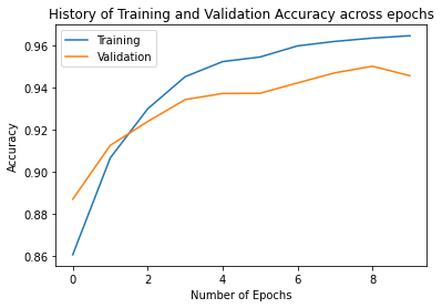
Visualizing the history

import matplotlib.pyplot as plot

plot.plot(history.history["accuracy"], label="Training")
plot.plot(history.history["val_accuracy"], label="Validation")
plot.legend(loc="upper left")
plot.ylabel("Accuracy")
plot.xlabel("Number of Epochs")
plot.title("History of Training and Validation Accuracy across epochs")

Text(0.5, 1.0, 'History of Training and Validation Accuracy across epochs')

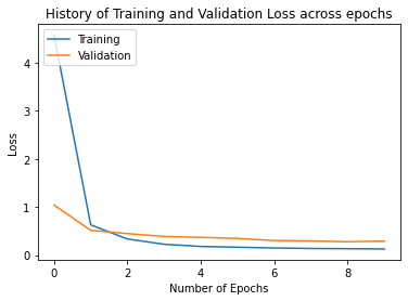
plot.plot(history.history["loss"], label="Training")
plot.plot(history.history["val_loss"], label="Validation")
plot.legend(loc="upper left")
plot.ylabel("Loss")
plot.xlabel("Number of Epochs")
plot.title("History of Training and Validation Loss across epochs")

Text(0.5, 1.0, 'History of Training and Validation Loss across epochs')

loss, accuracy = model.evaluate(ds_test, verbose=0)
print(f"accuracy: {accuracy} and loss:{loss}")

accuracy: 0.9455000162124634 and loss:0.2909369468688965

Prediction

# Creating a dataset for testing
ds_test = tfds.load("mnist", split="test[20%:]", as_supervised=True, shuffle_files=True)

# Creating a probability model for different classes for obtaining the probabilty
# for each class
probability_model = tf.keras.Sequential([model, tf.keras.layers.Softmax()])

# Creating batches
ds_test_batch = ds_test.batch(128)

# Prediction
predictions = probability_model.predict(ds_test_batch)

Obtaining the number of predictions made

print(len(predictions))

8000

Check the probability values for second prediction

print(predictions[1])

[0.08533739 0.08533739 0.08533739 0.08533739 0.08534175 0.08533739
 0.08533739 0.08533739 0.08533739 0.23195921]

Get the class with the highest probability

import numpy as np

print(np.argmax(predictions[1]))

9

Get the class with the highest probability for all the classes

predictedlabels = [np.argmax(predictions[i]) for i in range(len(predictions))]

Get the actual class or label from the test dataset.

data = ds_test.as_numpy_iterator()
testdata = list(data)
labels = [testdata[i][1] for i in range(len(testdata))]
print(labels[1])

9

Evaluate the prediction using a confusion matrix

confusionmatrix = tf.math.confusion_matrix(labels, predictedlabels, num_classes=10)
print(confusionmatrix)

tf.Tensor(
[[745   0   4   0   3  12   6   2   3   2]
 [  0 892   3   3   2   3   1   1  11   0]
 [  4   4 740  25   2   3   6  10  13   3]
 [  2   0   6 777   0  20   0   4   4   1]
 [  0   1   2   0 756   2  10   1   7  20]
 [  3   0   1  17   0 680   5   0   4   2]
 [  6   2   0   0   6   6 741   0   2   0]
 [  1   8  10  13   2   2   0 767   5  12]
 [  9   2   3  19   4  13   3   3 706   9]
 [  4   5   1  11  16  13   1   8   5 754]], shape=(10, 10), dtype=int32)

Visualizing the confusion matrix

import seaborn as sn

sn.heatmap(confusionmatrix)

<matplotlib.axes._subplots.AxesSubplot at 0x7f8e4ab4bf60>